

Load-pull is a measurement or simulation technique in which the load impedance presented to a power transistor is varied across the Smith chart while output power, efficiency, gain and linearity are recorded at each point. The results are drawn as contours that show which load gives the most power or the best efficiency. Power amplifier output matching networks are designed to present that load, not the conjugate of the transistor’s output impedance.
Small-signal amplifiers are matched for gain using S-parameters. A power amplifier is limited by how far its voltage and current can swing, so the best load is set by those limits. The load-line method developed by Cripps gives a first estimate from three numbers on the datasheet, and load-pull refines it with real device behaviour. This page covers both, then shows how harmonic terminations raise efficiency and how the output match is built, with a worked 12 W example. It is part of the RF amplifiers section of the RF design reference.
Why a power amplifier is not conjugately matched
A conjugate match delivers the maximum power that a linear source can supply. A transistor at high drive is not a linear source with a fixed internal impedance. Its output current cannot exceed a maximum value, Imax, and its drain voltage cannot fall below the knee voltage, Vk, or rise past breakdown. The output power is therefore limited by the signal swing that fits inside those boundaries, and the load that allows the largest swing of both voltage and current at the same time is usually much lower than the device’s small-signal output resistance.
The difference is large in practice. A device whose output resistance is 200 Ω and that is conjugately matched would reach its voltage limit at a current swing far below Imax. The worked example below shows that this costs more than 9 dB of output power compared with the correct load. That is why maximum available gain matching is the starting point for small-signal stages and the wrong target for the output of a PA.
The load-line (Cripps) method
For a device biased in class A or class B and driven to full swing, the fundamental drain current amplitude can reach Imax/2 and the fundamental voltage amplitude can reach VDD − Vk. The resistive load that allows both at once is
Ropt = (VDD − Vk) / (Imax/2) = 2(VDD − Vk) / Imax
and the maximum fundamental output power is
Pmax = ½ (VDD − Vk)(Imax/2)
In class A the device draws Imax/2 continuously and the drain efficiency is 50% × (VDD − Vk)/VDD. In class B the current is a half-sine with the same fundamental, so the same Ropt and Pmax apply, but the DC current falls and the efficiency rises to 78.5% × (VDD − Vk)/VDD, as explained in power amplifier classes.
Worked example: a 28 V device
Take a device with VDD = 28 V, Vk = 4 V and Imax = 2 A, and a small-signal output resistance of 200 Ω.
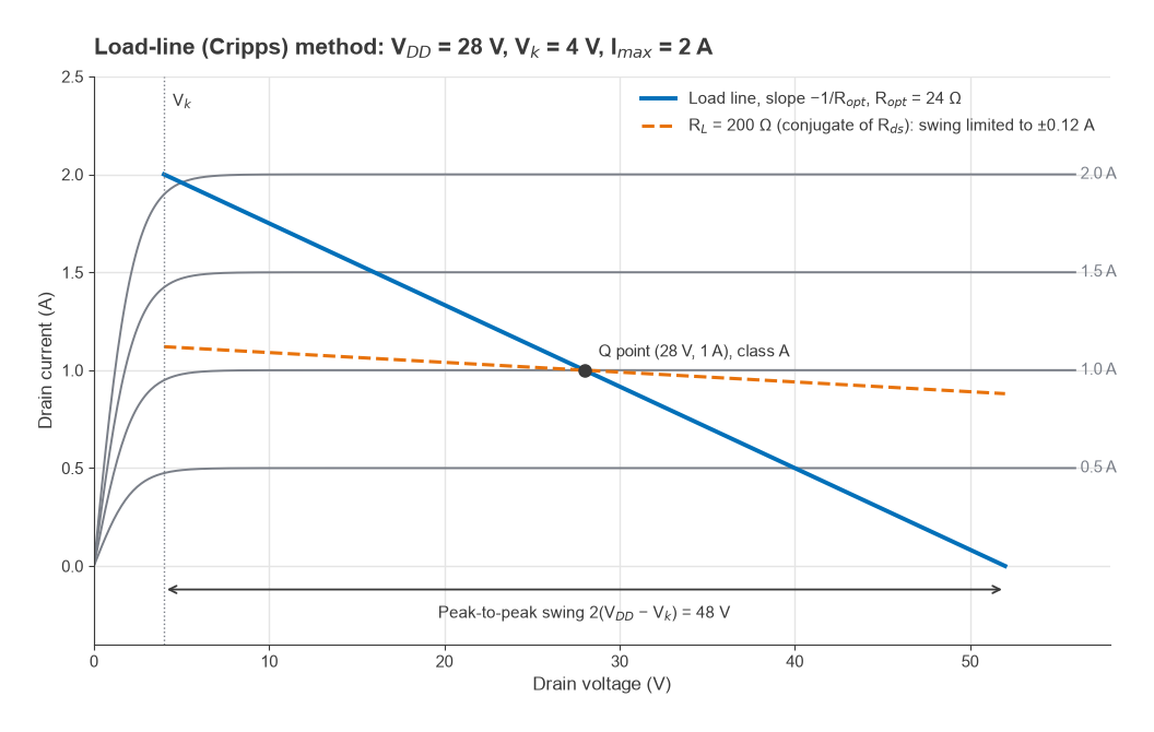
- Ropt = 2 × (28 − 4)/2 = 24 Ω.
- Pmax = ½ × 24 × 1 = 12 W, or 40.8 dBm.
- Drain efficiency at Pmax: 50% × 24/28 = 42.9% in class A; 78.5% × 24/28 = 67.3% in class B.
- With a conjugate match, 200 Ω, the voltage limit is reached first: P = (VDD − Vk)2/(2 × 200) = 242/400 = 1.44 W, or 31.6 dBm. That is 9.2 dB below Pmax, because the current swings only ±0.12 A of the ±1 A available.
Figure 1 shows both load lines on idealised I-V curves. The 24 Ω line runs from the knee at full current to 2VDD − Vk = 52 V at zero current, a peak-to-peak voltage swing of 48 V. In a real design, the peak drain voltage must also stay below the device’s breakdown rating with margin.
Load-pull contours
The load-line method gives one optimum point. Cripps extended it to contours of constant power. For a load Z = R + jX at the intrinsic drain, the fundamental current amplitude is limited to I1 = min(Imax/2, (VDD − Vk)/|Z|), and the output power is P = ½I12R. For loads with R below Ropt, the current limit applies and power falls in proportion to R. For loads with large |Z|, the voltage limit applies. A contour at power p × Pmax therefore runs from R = pRopt to R = Ropt/p on the real axis and is made of two arcs.
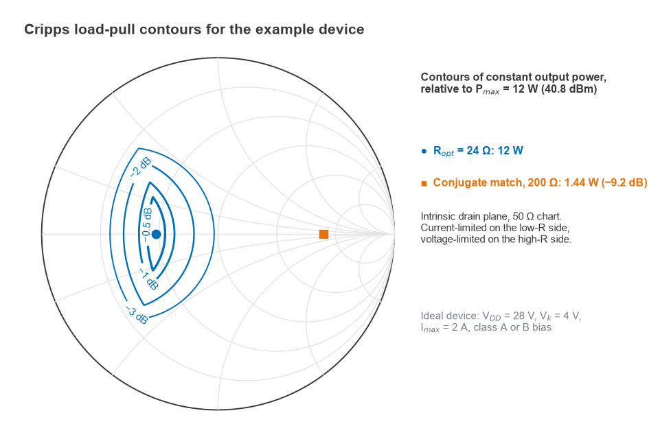
For the example device, the −1 dB contour (p = 0.794) spans 19.1 to 30.2 Ω along the real axis and allows reactance up to ±14.6 Ω at its low-resistance end. The −3 dB contour spans 12.0 to 47.9 Ω. Figure 2 plots the contours on a 50 Ω Smith chart. The conjugate-match point at 200 Ω lies far outside even the −3 dB contour.
Measured load-pull contours look broadly similar but differ in detail. Real devices have soft knees, nonlinear capacitances and thermal effects, so contours bend and shift with drive level and frequency. A load-pull system places the device between impedance tuners, either passive mechanical or electronic tuners or active loops that inject a signal back into the output, and steps the load across the chart. The output is a set of contours for output power, power-added efficiency (PAE), gain and often linearity metrics such as ACLR or AM-PM. The optimum loads for power and for efficiency are usually different, and the design load is chosen as a compromise between them. Harmonic balance simulation of a good large-signal model gives the same contours before hardware exists, as described in harmonic balance simulation.
Harmonic terminations
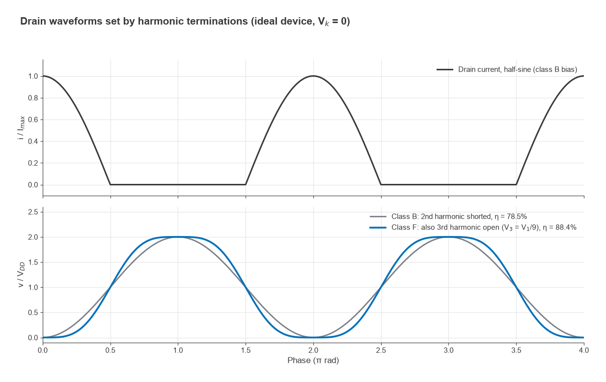
A class B, AB or C device produces drain current rich in harmonics. The impedances presented at 2f0 and 3f0 shape the drain voltage waveform, and through it the efficiency. Shorting the second harmonic keeps the voltage sinusoidal while the current is a half-sine; with an ideal device this gives 78.5% drain efficiency. Presenting an open circuit at the third harmonic as well allows a third-harmonic voltage component that flattens the voltage waveform. With the maximally flat choice V1 = 1.125VDD and V3 = V1/9, the efficiency becomes
η = ½ × (V1/VDD) × (I1/IDC) = ½ × 1.125 × π/2 = 88.4%
This is the third-harmonic-peaking class F amplifier. Figure 3 compares the two waveforms. Adding more harmonics pushes the theoretical limit higher, but each additional termination is harder to realise at the drain, because the device’s output capacitance shorts the higher harmonics. Inverse class F swaps the roles (second harmonic open, third short), and continuous modes such as class J use reactive harmonic terminations to widen bandwidth. In load-pull terms, harmonic load-pull measures how efficiency depends on the 2f0 and 3f0 impedances while the fundamental is held at its optimum. Harmonic content that escapes to the output must also be filtered, as covered in harmonic distortion and AM-PM.
Designing the output match
The load from the load-line method or from load-pull is defined at the intrinsic current source inside the device. Between that point and the package lead sit the drain-source capacitance and package parasitics, so the target must be translated to the package plane before the matching network is designed. Continuing the example with an output capacitance of 3 pF at 2 GHz:
- Intrinsic target: 24 Ω. The capacitance has susceptance ωC = 2π × 2×109 × 3×10−12 = 0.0377 S.
- The external load must have admittance 1/24 − j0.0377 S, so the load at the package plane is Z = 13.2 + j11.9 Ω. That is the impedance the matching network must present.
- One way to realise it: resonate the 3 pF with a shunt inductor, L = 1/(ω2C) = 2.11 nH. The bottom of this inductor can be bypassed to ground with a capacitor and used as the drain DC feed.
- Transform the remaining 24 Ω to 50 Ω with a low-pass L-network: Q = √(50/24 − 1) = 1.04, series L = QR/ω = 1.99 nH, shunt C = Q/(50ω) = 1.66 pF at the 50 Ω side. A circuit check confirms that the device sees 24.0 Ω at its current source.
- Add harmonic control. The low-pass network already presents a low impedance at harmonics, which approximates a second-harmonic short; a quarter-wave drain feed line or a resonant trap can set 2f0 and 3f0 more precisely.
- Simulate with the large-signal model, compare with load-pull data if available, and check stability, bandwidth, and peak voltages on all components.
Low transformation ratios like 24 to 50 Ω allow a single section. High-power devices often have optimum loads of a few ohms, which needs multi-section or tapered networks to cover useful bandwidth, as described under broadband matching. The Smith chart is the natural tool for each step. Bias networks follow the methods in RF amplifier biasing, and the heat generated at the drain is handled as in RF PA thermal design.
Frequently asked questions
What is load-pull?
Load-pull varies the load impedance presented to a transistor at large signal and records output power, efficiency, gain and linearity at each impedance. The results are plotted as contours on a Smith chart, from which the designer picks the load that best balances the performance goals.
How do you design a PA output match?
Find the optimum load, from the load-line formula Ropt = 2(VDD − Vk)/Imax or from load-pull data. Translate it through the device’s output capacitance and package parasitics to the package plane, then design a network that transforms 50 Ω to that impedance while controlling the harmonic impedances.
Why are the power and efficiency optimum loads different?
Maximum power needs the full current and voltage swing at once. Maximum efficiency favours a somewhat higher load resistance, which keeps the voltage swing high while lowering the current and its losses. Designers usually pick a load between the two optima.
What does a second harmonic short do?
It prevents a second-harmonic voltage from appearing at the drain, so a half-sine current produces a clean sinusoidal voltage. This allows class B operation to approach its theoretical 78.5% efficiency limit. Without it, the second-harmonic voltage distorts the waveform and either reduces the swing or raises peak voltage.
Related topics
Load-pull design builds on power amplifier classes, P1dB compression and RF transistor technologies. After the PA is designed, efficiency and linearity are traded off further with PA linearization, and the PA’s place in the radio is described in transmitter architectures. The section index is RF amplifiers, and terms are defined in the wireless terms glossary.