

AM-PM distortion is the change in an amplifier’s insertion phase as its input amplitude changes, so that the envelope of a modulated signal is converted into unwanted phase modulation. It is one of two memoryless signatures of a nonlinear amplifier, alongside AM-AM conversion (gain compression), and it rotates outer constellation points, raises EVM and spreads the spectrum into adjacent channels.
Harmonic distortion is the single-tone view of the same nonlinearity: energy appears at integer multiples of the input frequency, described by the second and third harmonic levels HD2 and HD3. This page covers both. It shows how harmonics follow from a power-series model and relate to the intercept points, then describes the AM-AM and AM-PM curves of solid-state and tube power amplifiers and what they do to a digitally modulated signal. It belongs to the linearity and distortion section of the RF design map.
Harmonics from a Power-Series Model
A weakly nonlinear, memoryless stage can be described by a polynomial transfer function
y(t) = a1x(t) + a2x2(t) + a3x3(t) + …
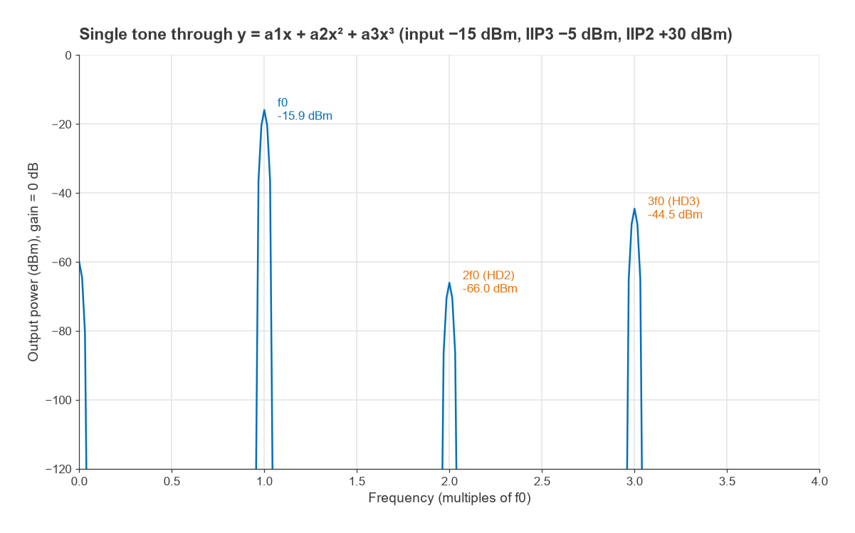
where a1 is the small-signal voltage gain and a2, a3 describe the curvature. For a single tone x(t) = A cos ωt, the trigonometric identities cos2θ = (1 + cos 2θ)/2 and cos3θ = (3 cos θ + cos 3θ)/4 give
- DC: a2A2/2
- Fundamental: (a1A + ¾a3A3) cos ωt
- Second harmonic: (a2A2/2) cos 2ωt
- Third harmonic: (a3A3/4) cos 3ωt
Even-order terms produce even harmonics and a DC shift; odd-order terms produce odd harmonics and also modify the fundamental. When a3 is negative, as it is in any amplifier that saturates, the ¾a3A3 term subtracts from the fundamental. That is the origin of gain compression and the 1 dB compression point. A perfectly balanced, symmetrical stage such as an ideal differential pair or push-pull amplifier cancels the even terms, which is why HD2 is a good indicator of balance and HD3 of the odd-order curvature that also drives intermodulation.
HD2 and HD3 Versus Drive Level
The harmonic levels are usually quoted in dBc, relative to the fundamental at the output. From the expressions above, the amplitude ratios at small signal are
HD2 = (a2/2a1) A HD3 = (a3/4a1) A2
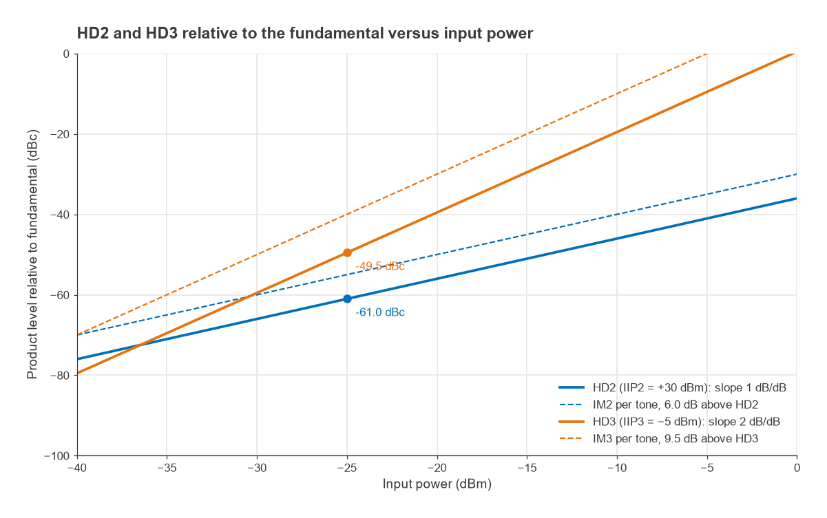
so in decibels HD2 rises 1 dB for every 1 dB increase in input and HD3 rises 2 dB per dB. Total harmonic distortion combines them as THD = √(HD22 + HD32 + …) using linear amplitude ratios.
Relation to IIP2 and IIP3
Datasheets normally give two-tone intercept points rather than polynomial coefficients. The same coefficients set both, so harmonics can be predicted from the intercept points. A two-tone third-order product has amplitude ¾a3A3, three times the third harmonic of a single tone of the same amplitude, and a second-order product at f1 + f2 has amplitude a2A2, twice the second harmonic. With input powers in dBm:
- HD2 (dBc) = Pin − IIP2 − 6.02 dB
- HD3 (dBc) = 2(Pin − IIP3) − 9.54 dB
The 6.02 dB and 9.54 dB terms are 20 log 2 and 20 log 3. They hold only while the stage is weakly nonlinear and memoryless. Harmonics also fall at frequencies two and three times higher, where the device gain and matching networks differ, so measured harmonics often depart from the prediction, sometimes by many decibels.
Worked Example: Harmonics of a Receiver Stage
Take an amplifier with IIP3 = −5 dBm and IIP2 = +30 dBm driven by a −25 dBm tone.
- HD3 = 2(−25 + 5) − 9.54 = −49.5 dBc. The two-tone IM3 at the same per-tone level would be −40 dBc.
- HD2 = −25 − 30 − 6.02 = −61.0 dBc. The IM2 product would be −55 dBc.
- THD = √(10−61.0/10 + 10−49.5/10) = 0.35 %, or −49.2 dBc, dominated by the third harmonic.
A numerical check, passing a sampled cosine through a polynomial with coefficients chosen to give these intercepts and taking an FFT, returns −60.9 dBc and −49.5 dBc. The small difference in HD2 comes from the slight compression of the fundamental by the cubic term. Raising the input by 10 dB to −15 dBm, as in Figure 1, pushes HD3 to about −29 dBc and compresses the fundamental by roughly 0.9 dB, a sign that the stage is no longer weakly nonlinear.
Harmonics at the Power Amplifier Output
In a transmitter the concern is the absolute harmonic power radiated, not its dBc value. Spurious emission rules are typically written as an absolute level, so the required filter rejection follows from simple subtraction. Suppose a PA delivers +30 dBm with HD2 = −25 dBc, a plausible value for a saturated single-ended stage, and the design target for harmonics is −30 dBm. The second harmonic sits at +5 dBm, so the output network must attenuate 2f0 by at least 35 dB, plus margin for temperature and part tolerance. That rejection is normally provided by the output matching network and a low-pass harmonic filter, designed with the methods in LC filter design. The PA class matters here: switching and saturated classes produce strong harmonics by design and rely on harmonic terminations to shape the waveforms.
AM-AM and AM-PM Curves of Power Amplifiers
A polynomial describes mild nonlinearity well but cannot follow an amplifier into saturation. For modulated signals near full power the device is instead characterised by two curves measured with a swept-power single tone:
- AM-AM: output amplitude versus input amplitude. It is linear at low drive, bends through the compression point and flattens at saturation.
- AM-PM: output phase relative to the small-signal phase, versus input amplitude. It is usually quoted as a slope in degrees per dB near a stated output power, or as the total phase change from small signal to a given compression level.
Together these define a complex gain G(A) = |G(A)| ejΦ(A) that depends only on the instantaneous envelope amplitude. Applied to a signal x(t) = A(t) ejθ(t), the output is |G(A(t))|A(t) ej(θ(t) + Φ(A(t))). Envelope variations therefore modulate both the output amplitude and the output phase.
Behavioural Models
Two classic memoryless models capture the shapes. Saleh’s model, fitted originally to travelling-wave tube amplifiers (TWTAs), uses
Aout(r) = αar / (1 + βar2) Φ(r) = αφr2 / (1 + βφr2)
with the frequently quoted parameters αa = 2.1587, βa = 1.1517, αφ = 4.0033 and βφ = 9.1040 for normalised amplitudes. Output saturates at r = 1/√βa = 0.93, where the phase shift has reached 22.4°, and the phase tends to αφ/βφ = 0.44 rad, or 25.2°, at high drive. Six decibels below that normalised input, the AM-PM slope is about 1.2° per dB.
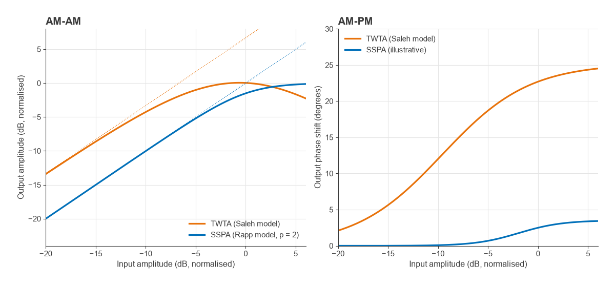
Rapp’s model is used for solid-state amplifiers (SSPAs):
Aout(r) = g r / [1 + (g r / Asat)2p]1/(2p)
The smoothness factor p sets how abruptly the curve moves from linear to saturated; large p approaches a hard limiter. The basic Rapp model has no AM-PM term, reflecting the fact that many solid-state amplifiers show much less phase conversion than tubes, typically a few degrees up to compression. That is a general tendency, not a rule. Bias point, device technology and harmonic terminations all change AM-PM, and class AB stages can show phase that first moves one way and then the other as drive increases.
Measuring the Curves
AM-AM and AM-PM are measured with a vector network analyser in power-sweep mode: S21 magnitude gives AM-AM and S21 phase gives AM-PM, both plotted against input or output power. A source power calibration is needed so that the swept power is known at the device input. Modulated-signal methods, which compare the captured output waveform with the known input, give the same curves as scatter plots and also reveal memory effects as spreading of the points. The general approach is covered in Radio Architectures Part 20 and VNA basics. In simulation, harmonic balance produces both curves and the harmonic levels from a single power sweep.
How AM-PM Shows Up in a Signal
A constant-envelope signal such as FM or GMSK sees a fixed phase offset, which is harmless. A signal with a varying envelope, such as QAM or OFDM, sees a phase that changes with every symbol. On a constellation diagram AM-AM pulls the outer points inward and AM-PM rotates them relative to the inner points.
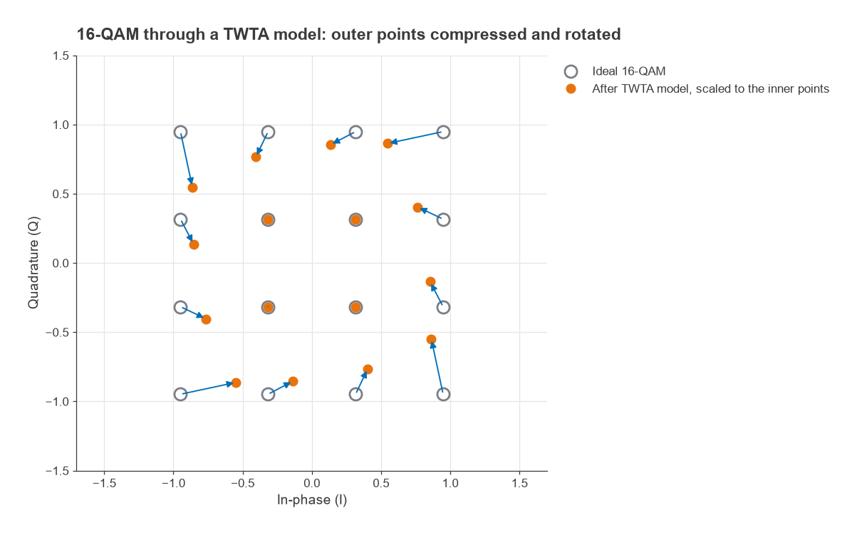
A simple estimate: in square 16-QAM the corner points have three times the amplitude of the inner points, a ratio of 9.54 dB. If the AM-PM slope were a constant 0.5° per dB over that range, the corners would rotate 4.77° further than the inner points. The resulting error vector is 2 sin(4.77°/2) = 0.083 of the corner amplitude, already a large contribution next to the few-percent EVM budgets of higher-order QAM.
Figure 4 applies the Saleh model to 16-QAM with the peak input at 0.56 on the normalised scale, about 4.4 dB below the saturating input. Referenced to the inner points, the corners lose 2.4 dB in amplitude and rotate by 12.6°. After the analyser removes the average gain and phase, the EVM is 9.4 %. The same mechanism spreads energy outside the channel, because AM-PM adds phase modulation whose bandwidth is set by the envelope rather than the original signal. That spreading appears as ACLR degradation and is part of the reason high-PAPR waveforms need back-off or PA linearization. Digital predistortion corrects AM-PM by applying the opposite phase rotation as a function of envelope amplitude, so a clean, repeatable AM-PM curve is easier to correct than a noisy one.
AM-PM and Intermodulation
The power-series model with real coefficients has no AM-PM at all. Allowing a3 to be complex adds a phase term proportional to A2, which is the small-signal form of AM-PM. A complex a3 still gives third-order products that rise 3 dB per dB, but their phase relative to the carrier changes, and when combined with even-order products and memory effects it causes the familiar asymmetry between the lower and upper IM3 tones. Cascaded stages add their distortion with phase, so the cascaded IP3 formulas assume the worst-case in-phase addition.
Frequently Asked Questions
What is AM-PM distortion?
AM-PM distortion is a change in an amplifier’s transmission phase that depends on the input amplitude. When the signal envelope varies, the phase of the output varies with it, adding unwanted phase modulation. It rotates outer constellation points, increases EVM and spreads energy into adjacent channels.
What is the difference between AM-AM and AM-PM?
AM-AM describes how output amplitude depends on input amplitude, which is gain compression. AM-PM describes how output phase depends on input amplitude. Both are measured with a swept-power tone and together form the complex gain of a memoryless amplifier model.
How are HD2 and HD3 related to IIP2 and IIP3?
For a weakly nonlinear stage, HD2 = Pin − IIP2 − 6.02 dB and HD3 = 2(Pin − IIP3) − 9.54 dB, both in dBc. The offsets arise because two-tone products are larger than single-tone harmonics for the same coefficients. Frequency-dependent gain and matching often make the real harmonics differ from these estimates.
Related Topics
See P1dB and gain compression for the AM-AM curve in detail, intermodulation and intercept points for two-tone behaviour, and PA linearization for correcting both curves. The linearity hub lists the remaining distortion topics, and the wireless terms glossary defines the abbreviations used here.