Wilkinson Power Divider: How It Works and How to Design One

A Wilkinson power divider is a three-port passive network that splits one input into two in-phase outputs while keeping all three ports matched and the two outputs isolated from each other. It does this with two quarter-wave lines of impedance √2·Z₀ (70.7 Ω in a 50 Ω system) and a 2Z₀ (100 Ω) resistor across the outputs. Run in reverse, the same circuit is a combiner.

The Wilkinson is one of the standard building blocks among RF passive components, and in the wider field of RF design it shows up wherever a signal has to be shared: LO distribution, phased-array feed networks, test setups and the combining of power amplifier stages. This page explains why the circuit works, how to design one step by step, and what limits its isolation and bandwidth.

Why a simple T-junction is not enough

A lossless, reciprocal three-port cannot be matched at every port, so a plain T-junction of 50 Ω lines leaves the outputs mismatched and coupled to each other. A resistive splitter fixes the match but costs 6 dB per path instead of 3 dB. The Wilkinson gets around that by adding a resistor that carries no current when the outputs are driven symmetrically, so it is lossless for the wanted signal and lossy only for signals that would otherwise travel between the outputs.

How the Wilkinson divider works

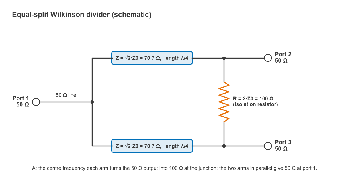
The equal-split divider has a 50 Ω input feeding a junction, two arms of characteristic impedance Z = √2·Z₀ and electrical length 90° at the centre frequency f₀, and a resistor R = 2Z₀ connected between the far ends of the arms, where ports 2 and 3 are taken off.

Quarter-wave 70.7 Ω arms and the 100 Ω resistor

Each arm is a quarter-wave transformer. A λ/4 line of impedance Z_T loaded by Z_L presents Z_in = Z_T² / Z_L at its input. With Z_T = 70.7 Ω and Z_L = 50 Ω:

Z_in = 70.71² / 50 = 5000 / 50 = 100 Ω

Two 100 Ω inputs in parallel at the junction give exactly 50 Ω, so port 1 is matched. By symmetry, port 2 and port 3 carry equal voltages with the same phase, no current flows in the resistor, and the input power divides equally: |S₂₁| = |S₃₁| = 1/√2, which is −3.01 dB. Both outputs lag the input by 90°.

Schematic of an equal-split Wilkinson divider with two 70.7 ohm quarter-wave arms and a 100 ohm resistor — Figure 1: Equal-split Wilkinson divider (schematic only). Each 70.7 Ω arm transforms 50 Ω to 100 Ω at the junction.

Even-mode and odd-mode analysis

The output match and isolation follow from splitting any excitation at ports 2 and 3 into an even mode (equal voltages) and an odd mode (opposite voltages).

Even mode. The midline of the circuit is a virtual open, so no current flows through the resistor. Looking into port 2, the 70.7 Ω λ/4 arm is terminated by 2Z₀ = 100 Ω (half of the split source), and transforms it to 70.71² / 100 = 50 Ω. Port 2 is matched.
Odd mode. The midline is a virtual ground. The junction end of each arm is shorted, and a shorted λ/4 line looks like an open circuit at port 2. What remains is half the resistor, R/2 = 50 Ω, to ground. Port 2 is matched again.

Because ports 2 and 3 are matched in both modes and the odd-mode energy is absorbed in the resistor, a signal entering port 2 reaches port 1 (losing 3 dB) but none of it arrives at port 3. That is the isolation. At f₀, the ideal S-matrix is:

S = (−j/√2) × [[0, 1, 1], [1, 0, 0], [1, 0, 0]]

The zeros on the diagonal are the port matches, and the zeros at S₂₃ and S₃₂ are the isolation. The full S-parameter description is what a simulator or a vector network analyzer reports for a real divider.

How to design a Wilkinson divider step by step

The design sequence is short.

Set the system impedance Z₀, the centre frequency f₀ and the band over which match and isolation must hold.
Choose the split ratio. For an equal split the arms are √2·Z₀ and R = 2Z₀.
Decide the number of sections. One section covers roughly a 1.4:1 band at 20 dB; wider bands need two or more sections.
Pick the substrate and calculate line widths and effective permittivity for each impedance with a microstrip calculator.
Compute the physical quarter-wave length, λ/4 = c / (4 f₀ √ε_eff), separately for each line width.
Lay out the arms so the resistor pads at ports 2 and 3 sit close together, and keep the outputs far enough apart that the arms do not couple.
Simulate with the resistor footprint and junction discontinuities included, then trim arm lengths to recentre the response.

Worked example: 2.4 GHz divider on a 0.508 mm laminate

Take Z₀ = 50 Ω, f₀ = 2.4 GHz, and a 0.508 mm hydrocarbon-ceramic substrate with a design permittivity of 3.66. Using the Hammerstad closed-form microstrip equations (zero-thickness copper, no dispersion):

Line	Impedance	Width	ε_eff	λ/4 at 2.4 GHz
Feed and outputs	50 Ω	1.12 mm	2.854	18.50 mm
Divider arms	70.7 Ω	0.60 mm	2.729	18.92 mm
Isolation resistor	100 Ω, placed across the arm ends

The arm length comes from λ/4 = 3 × 10⁸ / (4 × 2.4 × 10⁹ × √2.729) = 0.03125 / 1.652 = 18.92 mm. The narrower 70.7 Ω line has a lower effective permittivity than the 50 Ω line, so its quarter wavelength is slightly longer.

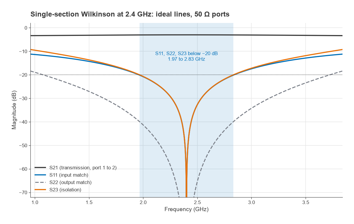
Simulated S21, S11, S22 and S23 of an ideal single-section 2.4 GHz Wilkinson divider versus frequency — Figure 2: Ideal single-section divider centred at 2.4 GHz. S11, S22 and S23 stay below −20 dB from 1.97 to 2.83 GHz.

Simulated with ideal lines, this divider has S₁₁, S₂₂ and S₂₃ all below −20 dB from 1.97 to 2.83 GHz, a fractional bandwidth of 0.86 / 2.4 = 36%. Insertion loss to each output stays within a few hundredths of a dB of the ideal 3.01 dB across that range. Conductor and dielectric loss on a real board typically add a few tenths of a dB.

Lumped-element version

At lower frequencies the arms get long, and each is often replaced by a lumped π-section with the same impedance and 90° phase shift. The values are L = Z/(2πf₀) and C = 1/(2πf₀Z). At 2.4 GHz with Z = 70.71 Ω, L = 70.71 / (2π × 2.4 × 10⁹) = 4.69 nH and C = 0.94 pF at each end of each arm. The two shunt capacitors at the input junction combine into 1.88 pF. The lumped version is smaller but narrower in bandwidth.

Isolation and bandwidth

At f₀ the ideal divider has perfect match and infinite isolation. Away from f₀ the arms are no longer 90° long, the transformation is no longer exact, and both degrade. Input match and isolation fall off at about the same rate, while the output match stays better for longer.

In practice, measured isolation on a single-section microstrip divider is limited by more than the arm length. The resistor has parasitic inductance and pad capacitance, the junction is not a point, and the two arms couple to each other if they run close together. Typical well-built single-section dividers achieve isolation in the 20 to 30 dB range across their band.

Multi-section dividers for wider bandwidth

Bandwidth grows by cascading quarter-wave sections in each arm with a resistor after every section, a method usually attributed to Cohn. For a two-section equal-split design centred at 2.4 GHz, the arms use about 82 Ω next to the input junction and 61 Ω next to the outputs. The resistor between the middle nodes is about 98 Ω and the resistor across the outputs is about 241 Ω. The product of the two arm impedances is 82 × 61 ≈ 5000, which preserves the 100-to-50 Ω transformation along each arm.

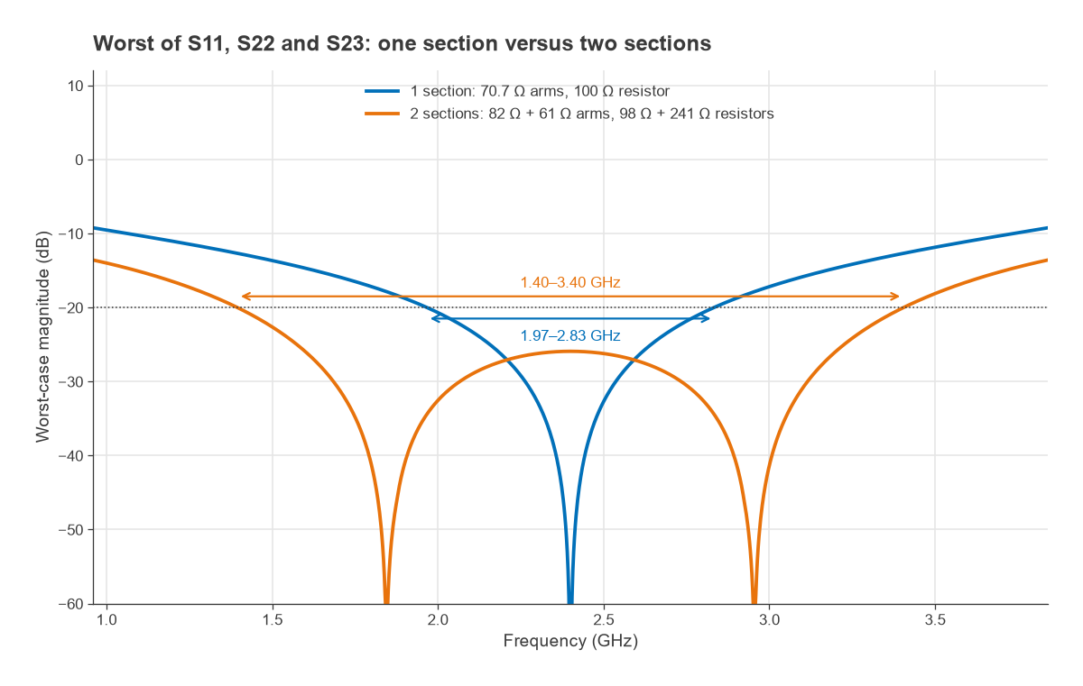
Worst-case match and isolation of one-section and two-section Wilkinson dividers versus frequency — Figure 3: Worst of S11, S22 and S23 for one section (1.97–2.83 GHz below −20 dB) and two sections (1.40–3.40 GHz).

With ideal lines, that design keeps all three reflections and the isolation below −20 dB from 1.40 to 3.40 GHz, a 2.4:1 frequency ratio. The cost is twice the arm length, two resistors and slightly more loss.

Unequal splits and N-way dividers

For an unequal split with power ratio K² = P₃/P₂, the standard design equations are:

Z₀₃ = Z₀ √((1 + K²) / K³)
Z₀₂ = K² Z₀₃
R = Z₀ (K + 1/K)

The outputs are then terminated in Z₀K and Z₀/K, which are usually brought back to Z₀ with additional quarter-wave transformers. For a 2:1 power split in 50 Ω, Z₀₃ = 51.5 Ω, Z₀₂ = 103.0 Ω and R = 106.1 Ω, with output terminations of 70.7 Ω and 35.4 Ω.

An N-way divider uses N arms of √N·Z₀ and N resistors of Z₀ tied to a common star point. Above N = 2 the star point is awkward to build in planar form, so large splits are normally built as trees of two-way dividers, as in the corporate feeds of a phased array. Where a 90° phase difference between outputs is needed instead of equal phase, a quadrature hybrid coupler is the usual choice.

Using the Wilkinson as a combiner

Two coherent, equal-amplitude, in-phase signals applied to ports 2 and 3 combine fully at port 1, and the resistor dissipates nothing. Any difference between the inputs, in amplitude or phase, appears as an odd-mode component that is dumped in the resistor. Two uncorrelated signals at different frequencies each lose 3 dB on their way to port 1.

This matters for combining power amplifiers. Take two 10 W amplifiers combined in phase: the output is 20 W and the resistor is idle. If one amplifier fails and presents a matched termination, the remaining 10 W splits evenly, 5 W to the output and 5 W into the resistor. The output drops by 10log(20/5) = 6.0 dB, and the resistor must be rated for that fault case, not for normal operation.

Practical layout notes

Use a small resistor package (0402 or smaller at microwave frequencies) and keep its pads short. The resistor and its pads are part of the odd-mode circuit.
Keep the two arms separated by at least three substrate heights where they run in parallel, to limit coupling between them.
Measure with all unused ports terminated in 50 Ω. An open or poorly matched output corrupts every other measurement.

Further reading on reducing the size of the arms is in the article on miniaturizing Wilkinson power dividers.

Frequently asked questions

How does a Wilkinson divider work?

Each 70.7 Ω quarter-wave arm transforms a 50 Ω output into 100 Ω at the input junction, and the two arms in parallel present 50 Ω to the source. When the outputs carry equal signals the resistor sees no voltage across it, so the split is lossless. Any signal that would pass from one output to the other is an odd-mode signal, and the resistor absorbs it.

Why is the isolation resistor 100 Ω?

In the odd mode the centre line of the circuit is a virtual ground, so each output port sees half the resistor to ground. Half of 100 Ω is 50 Ω, which matches the port. In general the resistor is 2Z₀ for an equal split.

Can a Wilkinson divider be used as a combiner?

Yes. Equal, in-phase signals at the two outputs combine without loss at the input. Unequal or out-of-phase components are dissipated in the resistor, so the combiner is efficient only when the inputs are well matched in amplitude and phase.