Directional Couplers: Coupling, Directivity and Design

A directional coupler is a passive four-port network that samples a known fraction of the power travelling in one direction on a transmission line while largely ignoring power travelling in the other direction. Power entering the input port passes mostly to the through port, a small fixed fraction appears at the coupled port, and ideally none reaches the isolated port. That directional selectivity is what separates a coupler from a simple power splitter.

Couplers are used wherever a circuit needs to measure or inject a signal without disturbing the main path: transmitter power monitors, reflectometers, vector network analyzers, feedback paths for automatic level control and predistortion, and test ports. This page defines coupling, isolation and directivity, works through numeric examples, and covers the two most common planar designs, the coupled-line coupler and the branch-line coupler. It is part of the RF passive components section of the RF design reference.

How a directional coupler works

Figure 1 shows the port naming used throughout this page. Port 1 is the input, port 2 the through (or transmitted) port, port 3 the coupled port and port 4 the isolated port. In a coupled-line coupler, two transmission lines run parallel for a quarter wavelength. A wave on the main line couples to the adjacent line through both the mutual capacitance and the mutual inductance between them. The capacitive and inductive contributions add in one direction along the coupled line and cancel in the other. In the common backward-wave design, the coupled signal emerges at the end nearest the input, and the far end of the coupled line is isolated.

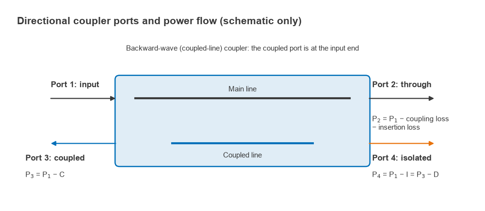
Four-port coupler diagram: input, through, coupled and isolated ports with power relations P3 = P1 - C and P4 = P3 - D — Figure 1: Schematic only. Port naming for a backward-wave coupler: input (1), through (2), coupled (3) and isolated (4), with the power relations for coupling, isolation and directivity.

The arrangement is symmetric. Power entering port 2, for example a wave reflected from a mismatched load, couples to port 4 instead of port 3. A coupler therefore separates forward and reverse waves, which is the property that makes reflection measurements possible. A useful theoretical result supports this: any lossless, reciprocal four-port that is matched at all ports is necessarily a directional coupler.

Coupling, isolation and directivity

With power P₁ applied at port 1 and all ports terminated in Z₀, the main specifications are defined as positive dB values:

Coupling: C = 10log₁₀(P₁/P₃) = −20log₁₀|S₃₁|
Isolation: I = 10log₁₀(P₁/P₄) = −20log₁₀|S₄₁|
Directivity: D = 10log₁₀(P₃/P₄) = I − C
Insertion loss: L = −20log₁₀|S₂₁|

Directivity measures how well the coupler distinguishes forward from reverse power. A coupler with 20 dB coupling and 50 dB isolation has 30 dB directivity: the wanted forward sample at port 3 is 30 dB stronger than the leakage at port 4. Directivity, not coupling, sets the accuracy of any reflection measurement made with the coupler, as the examples below show.

Coupling loss on the main line

Even a lossless coupler reduces the through power, because the sampled power has to come from somewhere. With voltage coupling factor c = 10^−C/20, the coupling loss is

L_c (dB) = −10log₁₀(1 − c²)

Coupling C (dB)	c	Coupling loss (dB)	Z_0e (Ω)	Z_0o (Ω)
3	0.708	3.02	120.9	20.7
6	0.501	1.26	86.7	28.8
10	0.316	0.46	69.4	36.0
20	0.100	0.044	55.3	45.2
30	0.032	0.004	51.6	48.4

A 20 dB coupler costs only 0.044 dB of coupling loss, which is why loosely coupled sensors are placed in transmitter outputs. Real couplers add conductor and dielectric loss on top of this figure. The even- and odd-mode impedances in the table are explained in the next section.

Coupled-line couplers

A pair of coupled lines supports two modes: an even mode, with both lines at the same potential, and an odd mode, with opposite potentials. Each has its own characteristic impedance, Z_0e and Z_0o. For a quarter-wave coupled section matched to Z₀, the design equations are

Z₀ = √(Z_0eZ_0o), c = (Z_0e − Z_0o)/(Z_0e + Z_0o)

Z_0e = Z₀√((1 + c)/(1 − c)), Z_0o = Z₀√((1 − c)/(1 + c))

For a 20 dB coupler in a 50 Ω system, c = 0.1, giving Z_0e = 55.3 Ω and Z_0o = 45.2 Ω. Check: √(55.28 × 45.23) = 50.0 Ω and (55.28 − 45.23)/(55.28 + 45.23) = 0.100. The physical line width and gap that produce these impedances depend on the substrate and are found with a field solver or the coupled-line formulas used by microstrip calculators.

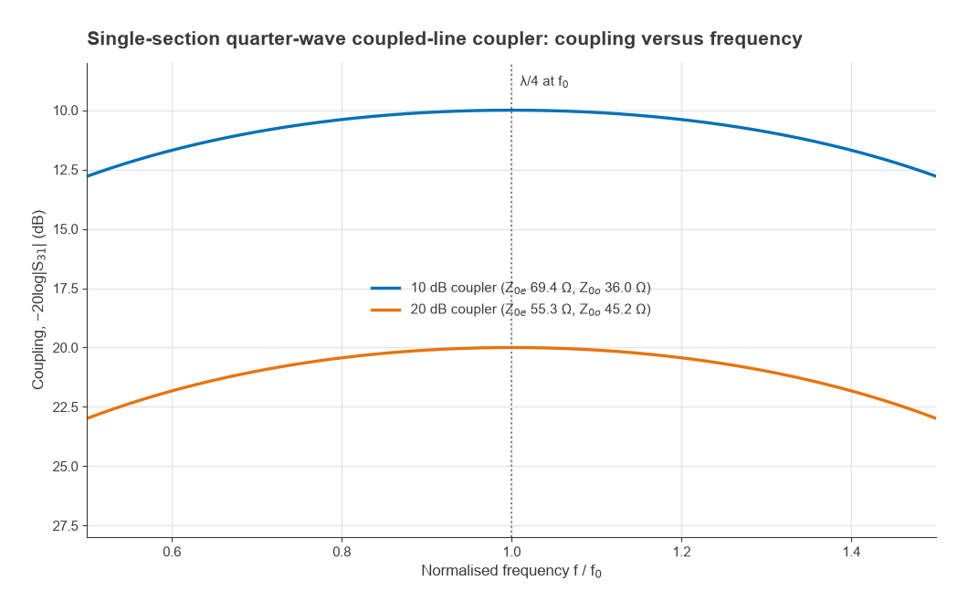
Coupling versus normalised frequency for single-section 10 dB and 20 dB coupled-line couplers, peaking at f0 — Figure 2: A single quarter-wave coupled section reaches its design coupling at f₀ and stays within 1 dB from about 0.69 f₀ to 1.31 f₀ (10 dB design).

The coupling of a single section varies with electrical length θ as

S₃₁ = jc sinθ / (√(1 − c²) cosθ + j sinθ)

Coupling peaks at the design value when θ = 90° (a quarter wavelength) and falls away on either side. Figure 2 shows that a single 10 dB section stays within 1 dB of nominal from about 0.69 f₀ to 1.31 f₀, and the 20 dB section from 0.70 f₀ to 1.30 f₀. Wider bandwidths use several cascaded sections with graded coupling.

Practical limits in microstrip

Two practical limits apply to edge-coupled lines. First, tight coupling needs a very small gap: a 10 dB coupler needs Z_0e/Z_0o of about 1.9, and a 3 dB coupler about 5.8, which is beyond what an etched gap can achieve. Tight couplings therefore use interdigitated Lange couplers or broadside-coupled lines in a multilayer board. Second, in microstrip the even and odd modes travel at different velocities, because the odd mode has more of its field in air. The capacitive and inductive coupling then no longer cancel exactly at the isolated port, and directivity in a simple microstrip coupler is often only around 10 to 20 dB. Stripline, with a homogeneous dielectric, does not have this problem. In microstrip, compensating capacitors at the ends of the coupled section, a dielectric overlay, or saw-tooth line edges can equalise the mode velocities and improve directivity.

Branch-line couplers

A branch-line coupler is made of four quarter-wave lines arranged in a square: two series arms of impedance Z_a along the main and coupled paths, and two shunt arms of impedance Z_b joining them. For a voltage coupling c in a Z₀ system,

Z_a = Z₀√(1 − c²), Z_b = Z_a/c

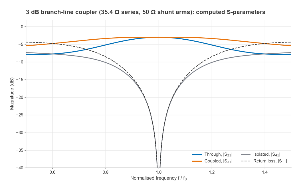
The 3 dB case, with c = 1/√2, gives Z_a = 35.4 Ω and Z_b = 50 Ω. Its through and coupled outputs are equal in amplitude and 90° apart in phase, so it is also a quadrature hybrid, covered further on the hybrid couplers page. Figure 3 shows its S-parameters computed from a nodal analysis of the four lines. At f₀ the through and coupled outputs are both −3.01 dB with a 90.0° phase difference, and the input match and isolation are ideal. The amplitude balance stays within 0.5 dB from 0.907 f₀ to 1.093 f₀, while isolation better than 20 dB holds only from 0.948 f₀ to 1.052 f₀, about 10% bandwidth.

Computed S21, S31, S41 and S11 of a 3 dB branch-line coupler from 0.5 to 1.5 f0, with deep isolation and match at f0 — Figure 3: Computed response of a 3 dB branch-line coupler (35.4 Ω series, 50 Ω shunt arms). Isolation exceeds 20 dB only from 0.948 f₀ to 1.052 f₀.

Branch-line couplers suit tight coupling. For loose coupling the shunt arms become impractical: a 10 dB design needs Z_b = 150 Ω, and a 20 dB design needs 497.5 Ω, far beyond what a printed line can realise. For couplings looser than about 10 dB, coupled-line designs are the normal choice.

Why directivity matters

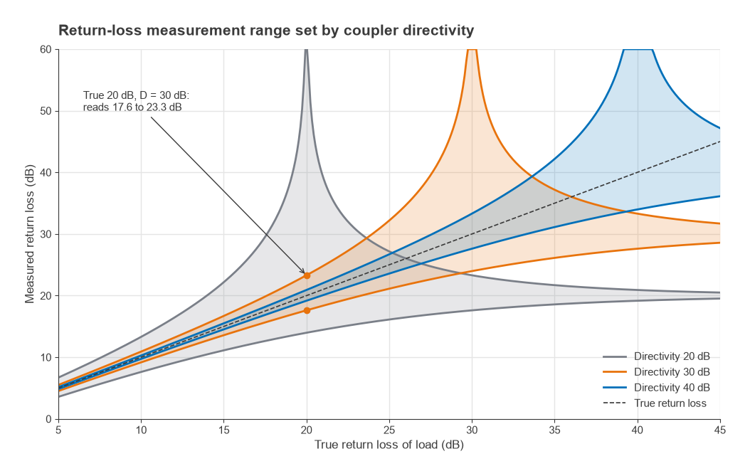
When a coupler is used to measure reflected power, the reading at the reverse port is the sum of the true reflected sample and the forward-wave leakage allowed by finite directivity. With a true reflection coefficient |Γ| and directivity leakage |Γ_D| = 10^−D/20, the measured value lies between |Γ| − |Γ_D| and |Γ| + |Γ_D|, depending on the relative phase.

Measured versus true return loss for 20, 30 and 40 dB directivity; true 20 dB reads 17.6 to 23.3 dB at 30 dB directivity — Figure 4: Finite directivity turns a return-loss reading into a range. A true 20 dB return loss measured with 30 dB directivity can read anywhere from 17.6 dB to 23.3 dB.

Worked example: return-loss measurement

A load has a true return loss of 20 dB (|Γ| = 0.100), measured through a coupler with 30 dB directivity (|Γ_D| = 0.0316). The measured reflection lies between 0.0684 and 0.1316, so the measured return loss lies anywhere from 17.6 dB to 23.3 dB. With 40 dB directivity the range narrows to 19.2 to 20.9 dB. With 20 dB directivity the leakage equals the true reflection, so a perfect cancellation can make the load appear perfectly matched while the worst case reads 14.0 dB (Figure 4). A rule of thumb follows: directivity should exceed the return loss being measured by at least 10 dB, and preferably 20 dB. Vector network analyzers remove most of this error through calibration, which measures the effective directivity and subtracts it vectorially.

Worked example: transmitter power monitor

A dual-directional 20 dB coupler with 25 dB directivity monitors a 40 dBm transmitter driving an antenna with VSWR 2:1. The reflection coefficient is (2 − 1)/(2 + 1) = 0.333, a return loss of 9.54 dB, so 30.46 dBm is reflected.

Forward sample: 40 − 20 = 20 dBm
Reflected sample: 30.46 − 20 = 10.46 dBm
Forward leakage into the reflected port: 40 − 20 − 25 = −5 dBm, 15.46 dB below the reflected sample
Reflected reading error: 20log₁₀(1 ± 10^−15.46/20) = +1.35 dB to −1.60 dB

For a VSWR alarm this accuracy is usually adequate. For a better-matched antenna the leakage would be a larger fraction of the reading, and a higher-directivity coupler would be needed. The samples are typically fed to RF power detectors, and the readings are often converted to VSWR or return loss in firmware.

Frequently asked questions

How does a directional coupler work?

Two transmission lines placed close together for a quarter wavelength couple through mutual capacitance and inductance. The two coupling mechanisms add for waves travelling in one direction and cancel for the other, so the coupled port samples only the forward wave while the reverse wave appears at the isolated port.

What is directivity?

Directivity is the ratio, in dB, of the power at the coupled port to the power at the isolated port for a signal applied to the input. It equals isolation minus coupling. It sets how accurately the coupler can separate forward from reflected power.

What is the difference between coupling and isolation?

Coupling is the attenuation from input to coupled port, the wanted sample. Isolation is the attenuation from input to isolated port, the unwanted leakage. A good coupler has isolation much larger than its coupling.

When should a branch-line coupler be used instead of a coupled-line coupler?

Branch-line couplers are practical for tight coupling, typically 3 to about 10 dB, and are simple to print. Coupled-line couplers handle loose coupling and offer wider bandwidth per section.