


Transmission lines are guided structures that carry RF energy between two points, and the main types are coaxial cable, parallel wire line, microstrip, stripline, coplanar waveguide and hollow waveguide. They differ in propagation mode, characteristic impedance, loss, usable frequency range, shielding and cost. The right choice depends mostly on frequency, power and whether the line sits on a PCB or between units.
This article compares the families and explains the characteristics used to judge them. For the underlying theory, start with the introduction to transmission line theory.
Key characteristics of a transmission line
Every line can be described by a small set of properties. Designers compare these first and look at construction details afterwards.
- Characteristic impedance (Z0): the voltage to current ratio of a travelling wave, set by geometry and dielectric.
- Propagation mode: the field pattern. TEM lines have no cutoff frequency, while hollow waveguide does.
- Velocity factor: phase velocity as a fraction of c, equal to 1/√εeff in non-magnetic lines.
- Attenuation: loss in dB per metre, growing with frequency. See transmission line losses and power handling.
- Power handling: the average limit from heating and the peak limit from voltage breakdown.
- Upper frequency limit: where higher-order modes or excessive loss end useful single-mode operation.
- Shielding: how well the fields are contained, which sets radiation and crosstalk.
The distributed values behind Z0 and velocity are covered in transmission line parameters.
Main types of transmission line
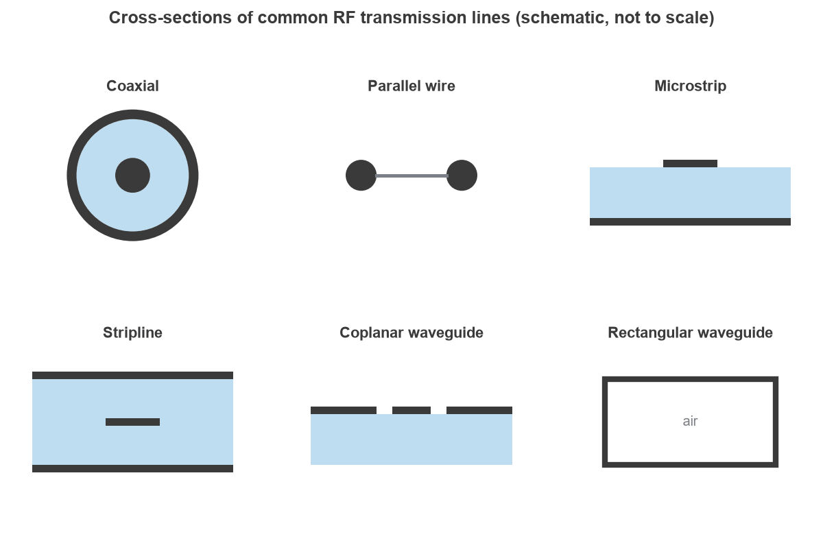
Figure 1 shows the cross-sections. The first five have two separate conductors and can carry DC. Hollow waveguide has one conductor and cannot.
Coaxial cable
A coaxial line has a centre conductor inside a concentric shield, with the fields confined to the dielectric between them. The mode is TEM, so the line works down to DC, and the good shielding makes coax the default between units. Its impedance is:
Z0 = (59.96 / √εr) ln(D/d)
where D is the inside diameter of the shield and d the diameter of the centre conductor. Flexible braided cable, semi-rigid tube and low-loss foam cable all follow this relation. RF connectors must preserve the same impedance, and they often set the upper frequency limit of a cable assembly.
Parallel wire line
Two wires held apart by a dielectric web or spacers form a balanced line. In air, Z0 = 119.9 acosh(D/d), where D is the centre spacing and d the wire diameter, and a D/d of 10 gives about 359 Ω. Parallel lines have low loss at HF and VHF but radiate and pick up nearby objects, so they are limited to feed lines at the lower frequencies and to balanced antenna systems.
Microstrip
Microstrip is a trace on a dielectric above a ground plane. Some of the field travels in air and some in the substrate, so the mode is quasi-TEM and εeff falls between 1 and εr. It is cheap, easy to probe and tune, and open on the top side, which allows some radiation and coupling. The microstrip calculator gives width against impedance. Microstrip is also the basis of many printed networks, including microstrip filters.
Stripline
Stripline places the trace between two ground planes inside the board. The field is fully in the dielectric, so the mode is close to pure TEM, and isolation between traces is high. For the same impedance the trace is narrower than microstrip, which raises conductor loss, and components must be reached through vias.
Coplanar waveguide
Coplanar waveguide puts ground on both sides of the trace on the same layer, usually with a further ground plane below. Short ground returns and easy shunt mounting suit it to millimetre-wave circuits, wafer probing and antenna feeds. Stitching vias must be spaced closely to suppress unwanted modes.
Rectangular waveguide
A waveguide is a hollow metal tube that carries TE and TM modes above a cutoff frequency set by its width. With a large conductor surface and an air interior, it offers very low loss and high power handling. The costs are size, weight, a limited bandwidth of well under an octave for single-mode operation, and rigid mechanical mounting.
Comparison of transmission line types
The table gives typical, approximate ranges. Actual limits depend on size, materials and construction.
| Type | Mode | Typical Z0 | Typical use | Main limitation |
|---|---|---|---|---|
| Coaxial cable | TEM | 50 or 75 Ω | DC to tens of GHz, between units | Loss in small cable, TE11 limit |
| Parallel wire | TEM | 100 to 600 Ω | HF and VHF feed lines | Radiation, poor shielding |
| Microstrip | Quasi-TEM | 20 to 120 Ω | PCB lines to tens of GHz | Radiation, dispersion |
| Stripline | TEM | 30 to 100 Ω | Multilayer PCB, isolated routing | Higher loss, via access |
| Coplanar waveguide | Quasi-TEM | 40 to 100 Ω | Millimetre-wave circuits, probing | Unwanted modes without vias |
| Waveguide | TE or TM | No single value | Roughly 1 GHz to beyond 100 GHz, high power | Size, cutoff, narrow band |
Coaxial design example
Worked example: impedance and limits of a semi-rigid coax
Consider a semi-rigid cable with a centre conductor of d = 0.91 mm, a shield inside diameter of D = 2.98 mm and solid PTFE dielectric with εr = 2.03.
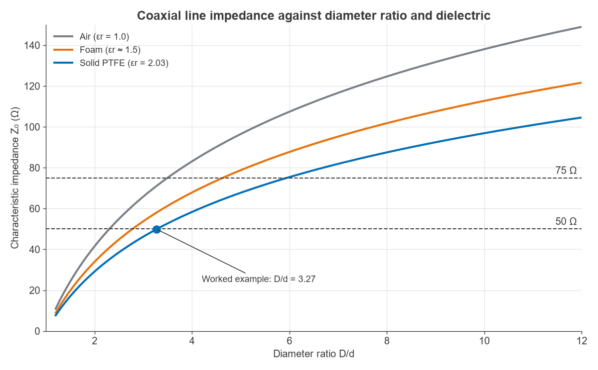
- Diameter ratio: D/d = 2.98 / 0.91 = 3.27.
- Impedance: Z0 = (59.96 / √2.03) × ln 3.27 = 49.9 Ω.
- Velocity factor: 1 / √2.03 = 0.702, which gives a delay of 4.75 ns/m.
- Per-unit-length values: C = 2πε / ln(D/d) = 95.2 pF/m and L = (μ0 / 2π) ln(D/d) = 237 nH/m.
The upper limit comes from the first higher-order mode, TE11. Its cutoff is approximately:
fc ≈ c / (π × (D + d)/2 × √εr)
With these dimensions, fc ≈ 34.4 GHz. Above it, energy can travel in more than one mode with different velocities, so practical assemblies stay below it. Reducing the diameter raises the limit but also raises loss, which is why millimetre-wave cable is thin and lossy.
Figure 2 shows the same formula across a wider range. For PTFE, 50 Ω needs D/d = 3.28 and 75 Ω needs D/d = 5.94. The worked cable falls just below the first value because its dimensions are rounded.
How to choose a transmission line
A few questions narrow the choice quickly.
- Between boxes or units? Use coax, or waveguide at high power or high millimetre-wave frequencies.
- On a PCB, outer layer? Use microstrip for ordinary RF routing, or coplanar waveguide when a tight ground return or millimetre-wave performance matters.
- On a PCB, inner layer? Use stripline where isolation matters more than conductor loss.
- Very high power with low loss? Use waveguide if the bandwidth and size suit it.
- Balanced HF antenna feed? Parallel line remains a fair option, with care around nearby metal.
On a PCB the substrate strongly influences loss and impedance control, as the FR-4 versus Rogers comparison explains.
Frequently asked questions
What is the difference between microstrip and stripline?
Microstrip has a single ground plane under the trace, with some field in the air above. Stripline has ground planes on both sides, with all the field in the dielectric. Microstrip is easier to reach and tune, and stripline offers better isolation and a mode closer to TEM.
Why does a waveguide not work at low frequencies?
A hollow guide has one conductor, so it cannot carry a TEM wave. Fields fit inside it only when the wavelength is short enough, and below the cutoff frequency they decay instead of propagating. For a rectangular guide, the dominant mode cuts off when the wide wall is half a wavelength across.
Why do coaxial cables have an upper frequency limit?
Above the TE11 cutoff, a second mode can propagate and the single, well-defined impedance is lost. Loss in the conductor and dielectric, and the limits of the connectors, often set a lower practical limit first.
What does velocity factor tell a designer?
It gives the speed of the wave relative to light, and therefore the physical length of a given electrical length. A stub cut for 0.70 velocity factor is 30 percent shorter than its length in air. The wave propagation article goes further into this.
Related topics
For behaviour at the end of a line, see transmission line terminations and reflection and transmission coefficients. The general concepts are collected under RF fundamentals, and impedance at each interface can be checked using the VSWR and return loss calculator.