RF Power Detectors and Log Amps

An RF power detector is a circuit that converts the power of a radio-frequency signal into a DC or low-frequency voltage that a comparator, ADC or control loop can read. The three common families are diode detectors, which rectify the waveform; RMS detectors, which respond to the true mean-square power; and logarithmic amplifiers, whose output in volts is proportional to the input in dBm.

Detectors sit behind directional couplers in transmitter power control loops, at the input of receivers for automatic gain control, and inside test equipment that reports power or VSWR. They belong to the RF passive components and building blocks section of the RF design guide.

How an RF Power Detector Works

Every detector relies on a nonlinear element. A purely linear network cannot produce a DC output from a sinusoid because the average of a sine wave is zero. A diode, a transistor junction or a squaring cell distorts the waveform so that a DC term appears, and a low-pass filter (often called the video filter) strips off the RF and its harmonics. What differs between detector types is how the size of that DC term depends on the input: in proportion to power, to peak voltage, or to the logarithm of power.

The input power and the RF voltage are tied together by the load. For a sinusoid across a matched 50 Ω termination, the peak voltage is

V_pk = √(2 · P · Z₀)

so −30 dBm (1 µW) corresponds to 10.0 mV peak, −10 dBm to 100 mV and 0 dBm to 316 mV. Conversions between dBm, watts and volts are covered in dB and dBm explained.

Diode Detectors

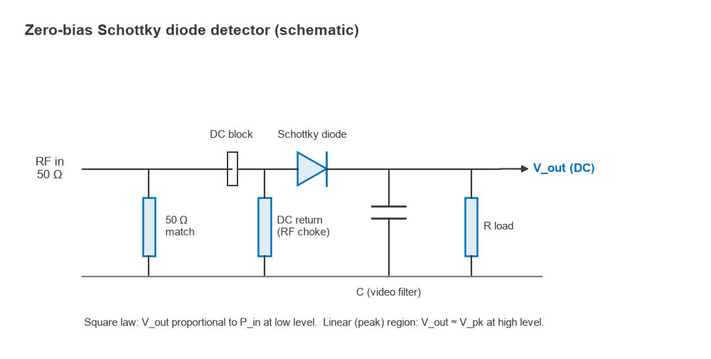
The simplest detector is a single Schottky diode followed by a capacitor. A 50 Ω resistor at the input sets the match, a DC return path keeps the diode’s average current from charging the input, and the capacitor holds the rectified voltage. Zero-bias Schottky diodes, with a low barrier height, are common because they need no bias current and therefore add no DC offset that drifts with temperature. Biased diodes respond faster but carry a DC offset that must be cancelled, often with a matched reference diode.

Schematic of a zero-bias Schottky diode detector with 50 ohm match, DC return, video filter capacitor and load — Figure 1: A zero-bias Schottky diode detector with input match, DC return path and video filter (schematic only).

Square-law and linear regions

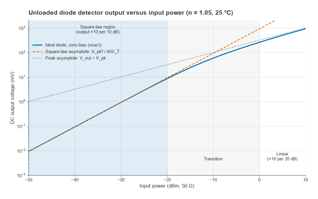
The diode current follows I = I_s[exp(V/nV_T) − 1], where n is the ideality factor and V_T = kT/q ≈ 25.85 mV at 25 °C. For an unloaded detector (the capacitor draws no current), the average diode current must be zero, which gives an exact result in terms of the modified Bessel function I₀:

V_out = nV_T · ln I₀(V_pk / nV_T)

Two limits follow from this. When V_pk is much smaller than nV_T, the output reduces to V_out ≈ V_pk² / (4nV_T). Because V_pk² is proportional to power, the output voltage is proportional to input power: this is the square-law region, where 10 dB more input gives ten times more output voltage. When V_pk is much larger than nV_T, the diode behaves as a peak detector and V_out approaches V_pk less a small offset. Output voltage then rises tenfold for every 20 dB of input, as the RF voltage itself does.

Diode detector DC output in millivolts versus input power from -50 to +10 dBm with square-law and peak asymptotes — Figure 2: Output of an ideal unloaded diode detector (n = 1.05, 25 °C). At −30 dBm it gives 0.913 mV; at −10 dBm, 58.5 mV against 92.1 mV predicted by square law.

Worked example: zero-bias Schottky detector

Take an ideal diode with n = 1.05 at 25 °C, so nV_T = 27.1 mV, driven from a matched 50 Ω source.

At −30 dBm, V_pk = 10.0 mV. The square-law formula gives (0.010)² / (4 × 0.0271) = 0.921 mV; the exact Bessel result is 0.913 mV. The two agree within 1 %, and the voltage sensitivity is about 0.91 mV per µW.
At −20 dBm, V_pk = 31.6 mV. Square law predicts 9.21 mV; the exact output is 8.53 mV, 7 % low, so a square-law calibration would read 0.3 dB under the true power.
At −10 dBm, V_pk = 100 mV. Square law predicts 92.1 mV but the diode delivers 58.5 mV. Reading this with a square-law calibration would understate the power by 10·log(58.5/92.1) = 2.0 dB.

A real diode has junction capacitance, series resistance and a finite video load, all of which reduce the sensitivity below the ideal figure, so the absolute millivolt values above are upper bounds. The shape of the curve, and the location of the transition between roughly −20 dBm and 0 dBm, carries over to practical zero-bias detectors. Below the square-law region, sensitivity is limited by the diode’s thermal noise in the video bandwidth, which for typical zero-bias parts places the usable floor somewhere in the −50 to −60 dBm range.

Waveform dependence

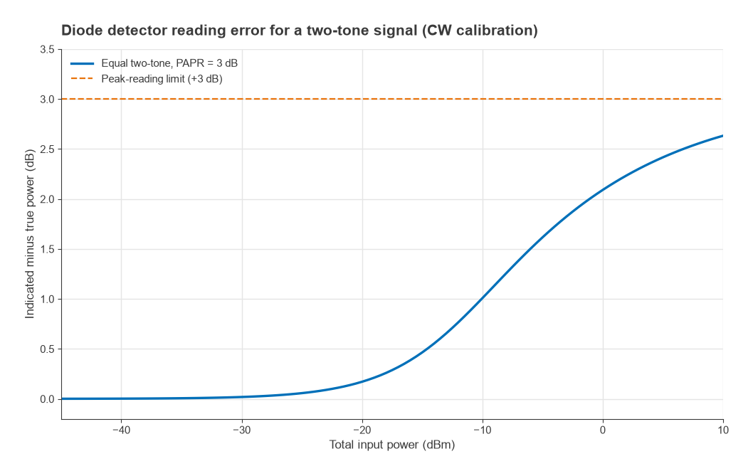
In the square-law region a diode detector measures the true average power of any waveform, because its output depends on the mean of v². In the linear region it tracks the peak instead. A signal with a high peak-to-average power ratio (PAPR) then reads high. For an equal-amplitude two-tone signal, whose PAPR is 3 dB, the error relative to a CW calibration is 0.02 dB at −30 dBm, 0.17 dB at −20 dBm, 1.0 dB at −10 dBm and 2.1 dB at 0 dBm, approaching the full 3 dB at high level. OFDM signals, with PAPR around 8 to 12 dB, make this worse, which is one reason detector choice is tied to the modulation; see modulation, EVM and PAPR.

Reading error of a CW-calibrated diode detector for a two-tone signal rising from 0 dB toward 3 dB with input power — Figure 3: Error of a CW-calibrated diode detector for an equal two-tone signal: 0.17 dB at −20 dBm, 1.0 dB at −10 dBm and 2.1 dB at 0 dBm.

RMS Detectors

An RMS detector is designed to produce an output proportional to the root-mean-square value of the input voltage, V_rms = √(mean v²), over a much wider range than a diode’s square-law region. Integrated RMS detectors typically use a squaring cell (or a translinear computing loop) followed by an averaging capacitor and a square-root or feedback stage. Because the output depends only on mean-square voltage, two signals with the same average power give the same reading whether they are CW, two-tone or a high-PAPR multicarrier waveform, provided the peaks stay inside the detector’s input range.

Some RMS detectors present a linear-in-volts output and others a linear-in-dB output; the latter combine RMS response with log-amp style scaling. The averaging capacitor sets the trade-off between residual ripple, which shows up as reading noise on signals with slow envelope variation, and response time. For a power-control loop that must settle within a transmit slot, that capacitor is often the dominant pole in the loop.

Logarithmic Amplifiers

A demodulating log amp produces an output that is linear in dB. The ideal transfer function is

V_out = V_slope · (P_in − P_intercept)

where V_slope is in mV/dB and P_intercept is the extrapolated input power at which the output would reach zero. Most use successive detection: a chain of limiting amplifiers, each with modest gain, with a detector at every stage output whose currents are summed. At low input, only the last stages contribute; as the input rises, each stage in turn saturates and its detector output reaches a fixed ceiling. Each 10 dB stage therefore adds roughly one fixed increment of output per 10 dB of input, and the sum approximates a logarithm with a small periodic ripple.

Worked example: successive-detection model

A simple numerical model uses eight limiting stages with 10 dB gain each (80 dB in total), a tanh limiting characteristic, and full-wave detectors on the input and every stage output. Scaling the summed output to a 25 mV/dB slope and fitting a line over −80 to −25 dBm gives an intercept of −102.6 dBm. The model stays within ±0.5 dB of the ideal line from −88.8 dBm to −24.3 dBm, a dynamic range of about 64 dB, and within ±1 dB from −92.5 dBm to −20.5 dBm.

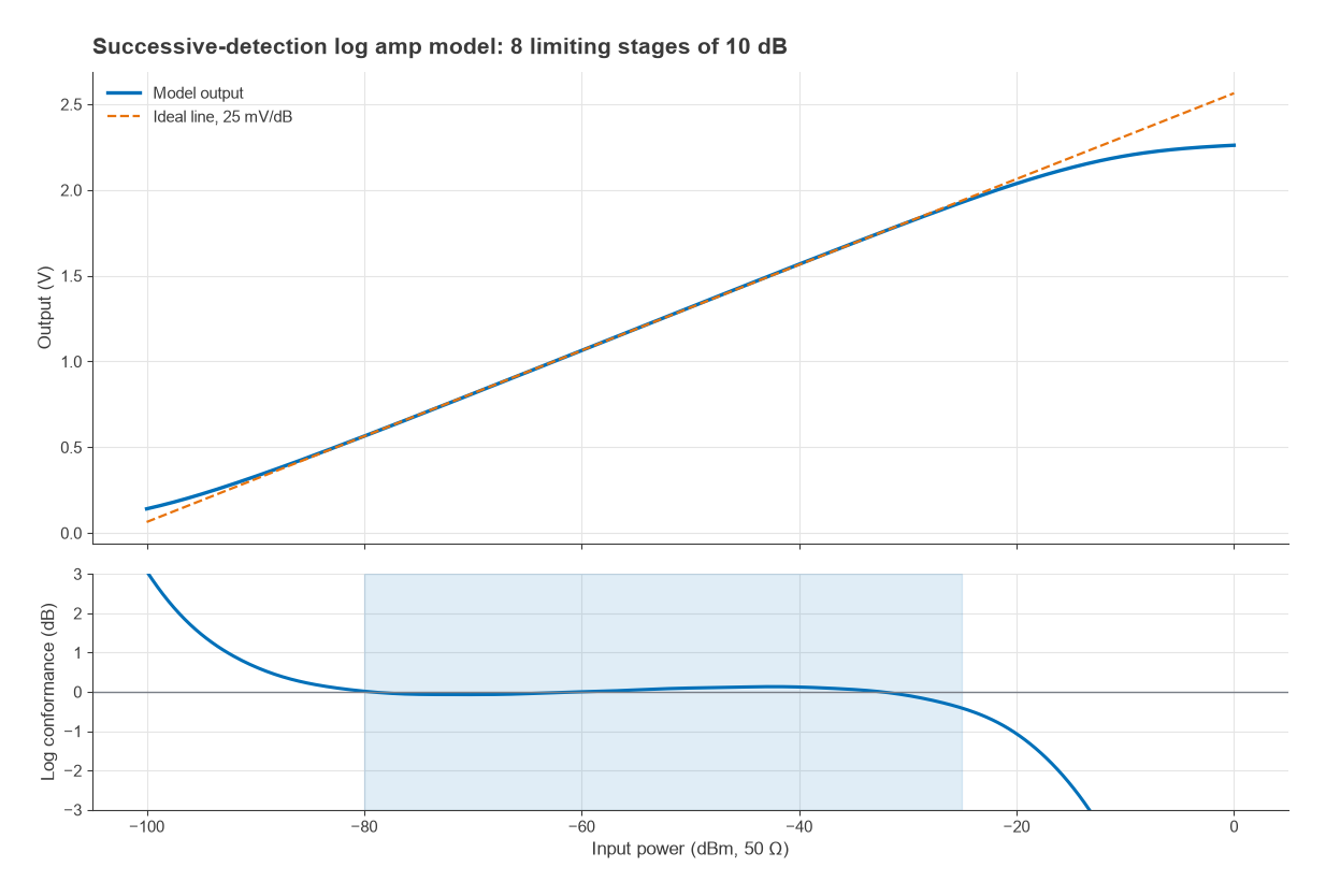
Log amp model output versus input power with ideal 25 mV per dB line and log conformance error below — Figure 4: Eight-stage successive-detection log amp model scaled to 25 mV/dB, intercept −102.6 dBm. Shaded: the −80 to −25 dBm fit range.

With that transfer function, an input of −40 dBm produces V_out = 0.025 × (−40 + 102.6) = 1.56 V. Working backwards, a reading of 0.9 V means P_in = −102.6 + 0.9/0.025 = −66.6 dBm. Firmware performs the same conversion on the ADC code, usually after a two-point calibration of slope and intercept on each unit.

Log amps respond to the envelope, not to true power, so their reading also shifts with waveform. The shift is roughly a constant number of dB for a given modulation format across most of the range, which makes it straightforward to correct once the format is known.

Comparing Detector Types

Property	Diode (zero-bias)	RMS detector	Log amp
Output law	Square law at low level, peak at high level	Proportional to V_rms (or dB of it)	Linear in dB
Typical dynamic range	About 30 to 50 dB usable	About 30 to 60 dB	About 50 to 100 dB
Waveform sensitivity	Low in square law, high in linear region	Low (true power)	Moderate, roughly constant offset
Response time	Very fast (ns possible)	Set by averaging capacitor	Fast (tens of ns typical)
Power and complexity	Passive, very simple	Active IC	Active IC
Typical use	Pulse and envelope detection, simple level sensing	PA power control with modulated signals	RSSI, AGC, wide-range monitoring

The ranges in the table are typical figures for the class, not limits for any particular device. Temperature drift affects all three. A diode detector’s sensitivity falls as nV_T rises with temperature, so precision designs add a reference diode or a temperature sensor and a correction table.

Detectors in a Power Control Loop

The classic transmitter arrangement places a directional coupler after the power amplifier, attenuates the coupled sample into the detector’s best range, and compares the detector output with a set-point. Suppose the PA delivers +30 dBm and the coupler has 30 dB coupling: 0 dBm appears at the coupled port. A 30 dB attenuator brings this to −30 dBm, inside the ±0.5 dB range of the log amp model above, which would read 0.025 × (−30 + 102.6) = 1.81 V.

Coupler directivity limits accuracy when the antenna mismatch is poor, because reflected power leaks into the forward-coupled port and adds to or subtracts from the reading. A second detector on the reverse-coupled port allows the loop to measure return loss as well, which is how many transmitters implement VSWR protection. For linearised amplifiers, detector accuracy directly affects how well the loop holds output power, which interacts with PA linearization.

Practical Design Notes

Match the detector input. A diode presents a high, level-dependent impedance; the 50 Ω termination in front of it sets the match and defines the voltage across the diode.
Calibrate at two or more points. Slope and intercept vary from part to part, and a diode’s curvature needs a table rather than a single gain constant.
Verify the loop against a thermal power sensor or a calibrated meter, as described in measuring amplitude and power in RF signals.

Frequently Asked Questions

How does an RF power detector work?

It passes the RF signal through a nonlinear element, such as a diode or a squaring cell, which creates a DC component related to the signal level. A low-pass filter removes the RF, leaving a voltage that depends on power, peak voltage or the logarithm of power, depending on the detector type.

What is the square-law region of a diode detector?

It is the low-level range, roughly below −20 dBm for a zero-bias Schottky diode, where the output voltage is proportional to input power. In that region the detector reads true average power regardless of waveform. Above it the diode becomes a peak detector.

What is the difference between an RMS detector and a log amp?

An RMS detector responds to mean-square voltage and so reads the same power for any waveform shape. A log amp responds to the signal envelope and gives an output linear in dB over a very wide range, but its reading shifts by a waveform-dependent offset.