RF Transistor Technologies: GaAs, GaN, SiGe, LDMOS and CMOS Compared

RF transistor technologies are the semiconductor processes, such as GaAs, GaN, SiGe, LDMOS and CMOS, that set a device’s speed, breakdown voltage, power density and noise. In the GaN vs GaAs comparison, neither is better overall: GaN wins on output power, voltage and ruggedness, while GaAs pHEMTs still offer slightly lower noise and lower cost at modest power levels.

The choice of process is one of the earliest decisions in RF design, because it fixes what the matching networks, bias circuits and thermal design must cope with. This page belongs to the RF amplifiers section. It compares the main technologies on the figures of merit that matter to amplifier designers, explains why GaN has taken over high-power amplifiers, and works through the load-line arithmetic that makes the difference concrete.

The Figures of Merit That Separate Technologies

Four numbers describe most of what an RF designer needs to know about a transistor process.

Transition frequency f_T: the frequency at which short-circuit current gain falls to unity. For a FET, f_T ≈ g_m / (2π(C_gs + C_gd)).
Maximum oscillation frequency f_max: the frequency at which unilateral power gain falls to unity. A common approximation is f_max ≈ (f_T / (8πR_gC_gd))^1/2, so gate or base resistance matters as much as raw speed. Useful amplifier gain is usually available up to roughly f_max/3.
Breakdown voltage: the drain-source or collector-emitter voltage the device survives. It sets the usable supply voltage and therefore the voltage swing.
Power density and minimum noise figure: watts per millimetre of gate periphery for power devices, and NF_min at a given frequency for low-noise devices.

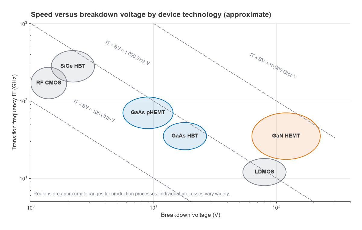
Speed and breakdown pull against each other. A short channel or thin base makes a device fast, but it also means the full supply voltage appears across a short distance, so the field reaches the material’s critical value sooner. The product f_T × BV therefore tends to be roughly constant for a given material, a relationship known as the Johnson limit. Using textbook values of critical field and saturation velocity, E_cv_sat/2π is roughly 480 GHz·V for silicon, 640 GHz·V for GaAs and 13,000 GHz·V for GaN. Real devices do not sit exactly on these lines, because breakdown definitions and device structures differ, but the factor of about 20 to 30 between GaN and the older materials is the root of its advantage.

Material Properties Behind the Differences

GaN and SiC are wide-bandgap materials. A bandgap of about 3.4 eV for GaN against 1.12 eV for silicon and 1.42 eV for GaAs gives a critical electric field roughly ten times higher, so a GaN transistor of the same size can hold off far more voltage. GaAs has very high bulk electron mobility, which is why it dominated low-noise microwave devices for decades. GaN HEMTs rely on a two-dimensional electron gas at an AlGaN/GaN interface with a high sheet charge, which produces large current per millimetre at high voltage.

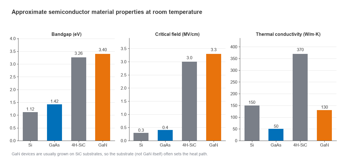
Bar charts of bandgap, critical field and thermal conductivity for Si, GaAs, 4H-SiC and GaN — Figure 1: Approximate room-temperature material properties. GaN’s bandgap of about 3.4 eV gives a critical field roughly ten times that of Si or GaAs.

Thermal conductivity is the other material property that matters for power. GaAs conducts heat poorly, at roughly a third of silicon’s value, which limits how much power can be concentrated in a small area. GaN is usually grown on silicon carbide substrates, and SiC conducts heat more than twice as well as silicon. That combination of high field strength and a good heat path is why GaN-on-SiC dominates high-power microwave amplifiers.

Comparison Table: GaAs, GaN, SiGe, LDMOS and CMOS

The table gives typical, approximate ranges for production processes as of 2026. Individual foundry processes vary widely, and a high-voltage variant of a process always trades away some speed, so treat these as orders of magnitude rather than specifications.

Technology	f_T / f_max (GHz, approx.)	Breakdown (approx.)	Power density (approx.)	NF_min (approx.)	Typical roles
RF CMOS (bulk and SOI)	150-350 / 200-400 in fine nodes	about 1-4 V per device; stacking raises it	low, well under 1 W/mm	below about 1 dB at a few GHz in fine nodes	Integrated transceivers, Wi-Fi, Bluetooth, mmWave beamformers, switches (SOI)
SiGe HBT (BiCMOS)	200-350 / 250-500	BV_CEO about 1.5-4 V	low	low, with low 1/f noise	mmWave front ends, radar chips, VCOs, high-speed data converters
GaAs pHEMT	40-120 / 100-200	about 8-15 V	about 0.5-1 W/mm	very low, a few tenths of a dB at 10 GHz for short gates	LNAs, gain blocks, switches, medium-power microwave PAs
GaAs (InGaP) HBT	30-60 / 50-100	BV_CEO about 10-20 V	moderate	moderate	Handset power amplifiers, gain blocks
GaN HEMT on SiC	20-100 / 50-200, depending on gate length	about 50-200 V or more	about 3-8 W/mm	low, typically somewhat above GaAs pHEMT	Base-station and radar PAs, rugged LNAs, wideband high-power amplifiers
Silicon LDMOS	10-20 / 20-30	about 65-110 V	about 1-2 W/mm	not used for low noise	High-power PAs below about 4 GHz, broadcast, ISM heating
InP HEMT and HBT	300-600 / 500-1,000 or more	about 2-5 V	low	lowest available at mmWave	Sub-THz and mmWave LNAs, cryogenic receivers, very high-speed circuits

Silicon CMOS and SiGe are fast but low voltage, and win where integration matters more than power. The compound semiconductors split into a low-noise branch (GaAs pHEMT, InP) and a high-power branch (GaN, with silicon LDMOS at lower frequencies).

Where each technology sits

Plotted as f_T against breakdown voltage, CMOS, SiGe and InP occupy the fast, low-voltage corner, GaAs the middle, and LDMOS and GaN the high-voltage side. Only GaN combines tens of gigahertz of f_T with breakdown above 100 V.

Log plot of transition frequency against breakdown voltage showing approximate regions for CMOS, SiGe, GaAs, GaN and LDMOS — Figure 2: Approximate fT and breakdown ranges for production processes, with constant fT × BV guide lines. GaN combines tens of GHz with breakdown above 100 V.

GaN vs GaAs: Which Is Better?

For power amplifiers above a few watts, GaN is usually the better choice. It runs from 28 V to 50 V supplies instead of about 5 V to 12 V, delivers several times the power per millimetre of gate, and tolerates mismatch and input overdrive that would destroy a GaAs device. The same ruggedness makes GaN LNAs attractive in receivers that must survive a nearby transmitter.

GaAs keeps its place in several areas. Short-gate GaAs pHEMTs reach slightly lower noise figure than comparable GaN devices, the processes are mature, and wafers are cheaper. At output powers below about a watt, GaN’s voltage advantage brings little benefit, and the higher bias voltage can be a burden in battery equipment. Handset PAs, for example, have largely stayed on GaAs HBT because they run from a single lithium cell. For most low-noise amplifier designs below about 20 GHz, GaAs pHEMT and SiGe remain the default, and the LNA selection guide covers how to compare candidates on noise and linearity.

Why GaN Is Used for Power Amplifiers

The advantage of high voltage shows up directly in the load line. For a class A or class B stage, the optimum load resistance that gives full voltage and current swing is

R_opt = (V_DD − V_k)² / (2P_out)

where V_k is the knee voltage and P_out is the fundamental output power. A higher supply raises R_opt with the square of the usable voltage swing. That moves the device impedance closer to 50 Ω, which makes the output match lower in loss and wider in bandwidth. The Bode-Fano limit discussed in broadband matching ties achievable bandwidth to the impedance transformation ratio, so a device that needs only a small ratio can cover more bandwidth.

Worked example: a 10 W output stage

Compare a GaAs pHEMT at V_DD = 5 V with V_k = 0.5 V and a GaN HEMT at V_DD = 28 V with V_k = 3 V, both delivering 10 W.

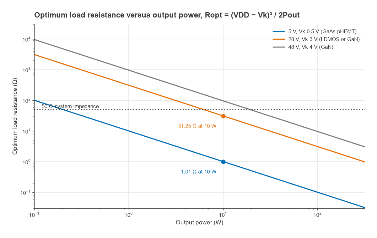
Optimum load resistance versus output power for 5 V, 28 V and 48 V supplies, with 10 W points at 1.01 and 31.25 ohms — Figure 3: Optimum load resistance from Ropt = (VDD − Vk)² / 2Pout. At 10 W a 5 V GaAs stage needs 1.01 Ω, a 28 V GaN stage 31.25 Ω.

GaAs: R_opt = 4.5² / 20 = 1.01 Ω. The peak current is I_max = 2(V_DD − V_k) / R_opt = 8.89 A, and the match must transform 50 Ω down by a ratio of about 49:1.
GaN: R_opt = 25² / 20 = 31.25 Ω. The peak current is 1.60 A, and the transformation ratio is only 1.6:1.
At 48 V with V_k = 4 V, a GaN device reaches R_opt = 96.8 Ω for the same 10 W, which is above 50 Ω.

The periphery needed follows from power density. At about 5 W/mm, a GaN device needs roughly 2 mm of gate width for 10 W. A GaAs pHEMT at about 0.8 W/mm needs roughly 12.5 mm, which means a much larger die, more parallel cells to combine and harder heat removal from a material with poor thermal conductivity. A 10 W GaAs stage is therefore usually built by combining several smaller devices.

GaN is not free of problems. Trapping effects cause current collapse and memory effects that complicate PA linearization, the devices need negative gate bias and correct bias sequencing, and the high power density makes thermal design the limiting factor in many designs. Characterising a GaN device usually requires load-pull, because the optimum load depends strongly on bias, frequency and drive.

SiGe, CMOS and LDMOS in Context

Silicon processes win wherever integration matters. CMOS puts a complete transceiver, digital logic included, on one die, and SOI CMOS is the standard process for antenna switches. SiGe BiCMOS adds fast, low 1/f noise bipolar transistors, which suits oscillators, mmWave front ends and radar chips. Both are covered further in RFIC design and in the MMIC vs RFIC comparison. At mmWave, phased arrays often pair silicon beamformer chips with compound-semiconductor front ends, a split described in mmWave radio architectures.

LDMOS is a laterally diffused silicon MOSFET built for high voltage. It is cheap, mature and rugged, and has long been the workhorse of base stations and broadcast transmitters below about 4 GHz. Its low f_T makes gain and efficiency fall off at higher frequencies, where GaN has taken share. Below 3 GHz the choice is mostly about cost, efficiency and bandwidth, and the power amplifier classes article explains how the operating class interacts with these device limits.

How to Choose a Technology

Lowest noise below about 20 GHz, discrete or MMIC: GaAs pHEMT, with SiGe as an integrated alternative. See the noise figure page for how device NF_min translates into system noise.
High power above about 3 GHz, or very wide bandwidth at high power: GaN on SiC.
High power below about 3 GHz at the lowest cost: LDMOS or GaN, depending on efficiency and bandwidth.
Full transceiver integration, high volume: CMOS or SiGe BiCMOS.
Battery-powered handset PA: GaAs HBT, or CMOS and SOI for lower-power standards.
Sub-THz LNAs and cryogenic receivers: InP.

Industry coverage of the shift is collected in the article on GaN RF taking market share in wireless infrastructure.

Frequently Asked Questions

GaN vs GaAs: which is better?

GaN is better for output power, supply voltage, bandwidth at high power and ruggedness. GaAs is often better for the lowest noise figure, low-voltage operation and cost at low power. The right choice depends on whether the circuit is a power amplifier or a low-noise stage.

Why is GaN used for PAs?

GaN’s high critical field allows supply voltages of 28 V to 50 V and power densities of several watts per millimetre. The high voltage raises the optimum load resistance, which makes the output match lower in loss and wider in bandwidth, and the SiC substrate removes heat well.

What is the difference between fT and fmax?

f_T is where current gain falls to one; f_max is where power gain falls to one. f_max depends on gate or base resistance and feedback capacitance as well as f_T, and it is the better guide to the highest frequency at which a device can amplify.