

An MMIC (monolithic microwave integrated circuit) is a single semiconductor die that contains a complete microwave function, such as an amplifier, mixer or switch, with all its transistors, matching elements and bias networks, usually built on a compound semiconductor such as GaAs, GaN or InP. An RFIC is a radio integrated circuit, usually in silicon CMOS or SiGe, that combines RF blocks with mixed-signal and digital circuits. Discrete design builds the same function from packaged transistors and passive parts on a printed circuit board.
The choice between the three is an integration level decision. It sets the achievable frequency and power, the development cost and time, the unit cost at volume, and how much can be changed after the first prototype. This page belongs to the RFIC design section of the RF design guide. It compares process technology, cost structure and frequency range, works through two numeric examples, and ends with a practical guide to when discrete design is still the right answer.
Three Levels of Integration
Discrete circuits use packaged transistors, chip inductors, capacitors and resistors connected by microstrip or coplanar lines on a PCB. Every element can be swapped with a soldering iron, and the transistor can be chosen from any vendor and process.
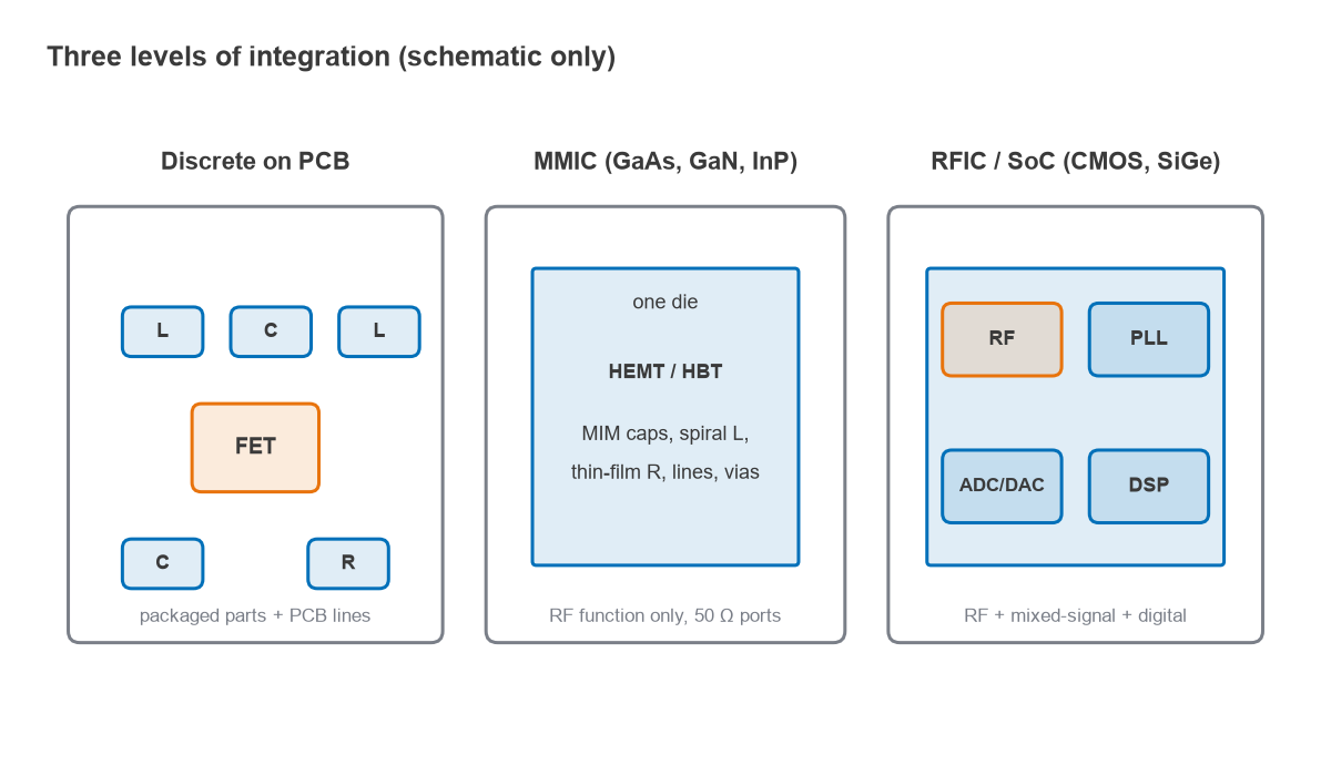
An MMIC puts the whole RF function on one die. Transistors are typically high electron mobility transistors (HEMTs) or heterojunction bipolar transistors (HBTs). Passives are metal-insulator-metal capacitors, spiral inductors, thin-film resistors and transmission lines on a semi-insulating substrate, with through-substrate vias to the backside ground. The die usually has 50 Ω RF ports and performs one function: a low-noise amplifier, a power amplifier, a switch, a mixer or a phase shifter.
An RFIC generally means a silicon chip, often a complete transceiver, where the RF front-end shares the die with synthesizers, data converters, calibration loops and digital control. A system-on-chip may add a processor and baseband. The defining advantage is that digital correction can compensate for analog weaknesses, which is what makes highly integrated zero-IF receivers and direct RF sampling designs practical.
Process Technology
The process sets the device speed, breakdown voltage, substrate loss and available passives. Silicon substrates in standard CMOS are conductive, so inductors and lines lose energy into the substrate and on-chip inductor Q is modest. Semi-insulating GaAs and the SiC substrates used for GaN behave much more like a low-loss dielectric, which helps passive Q and isolation between blocks. The broad positions below are approximate and change as processes improve; device details are compared in RF transistor technologies.
| Process | Typical role | Strengths | Limitations |
|---|---|---|---|
| Bulk CMOS | Transceiver RFICs, SoCs | Lowest cost at volume, digital integration | Low breakdown voltage, lossy substrate |
| RF SOI | Switches, front-end control, some LNAs | Stackable FETs, low parasitics, logic integration | Limited output power |
| SiGe BiCMOS | Radar, mmWave, high-performance transceivers | Fast HBTs with CMOS logic | Moderate power, higher wafer cost than CMOS |
| GaAs pHEMT / HBT | LNAs, PAs, switches, gain blocks | Low noise, good passives, mature MMIC process | Little digital integration |
| GaN HEMT | High-power PAs, rugged LNAs | High breakdown and power density | Cost, thermal design, bias sequencing |
| InP HEMT / HBT | Highest-frequency amplifiers | Very high device speed | Small wafers, high cost, low power |
Frequency and the Interconnect Problem
The higher the frequency, the more the connections between parts behave as circuit elements. A bond wire has an inductance of roughly 1 nH per millimetre, a common rule of thumb that varies with wire diameter and height. Its reactance is X = 2πfL.
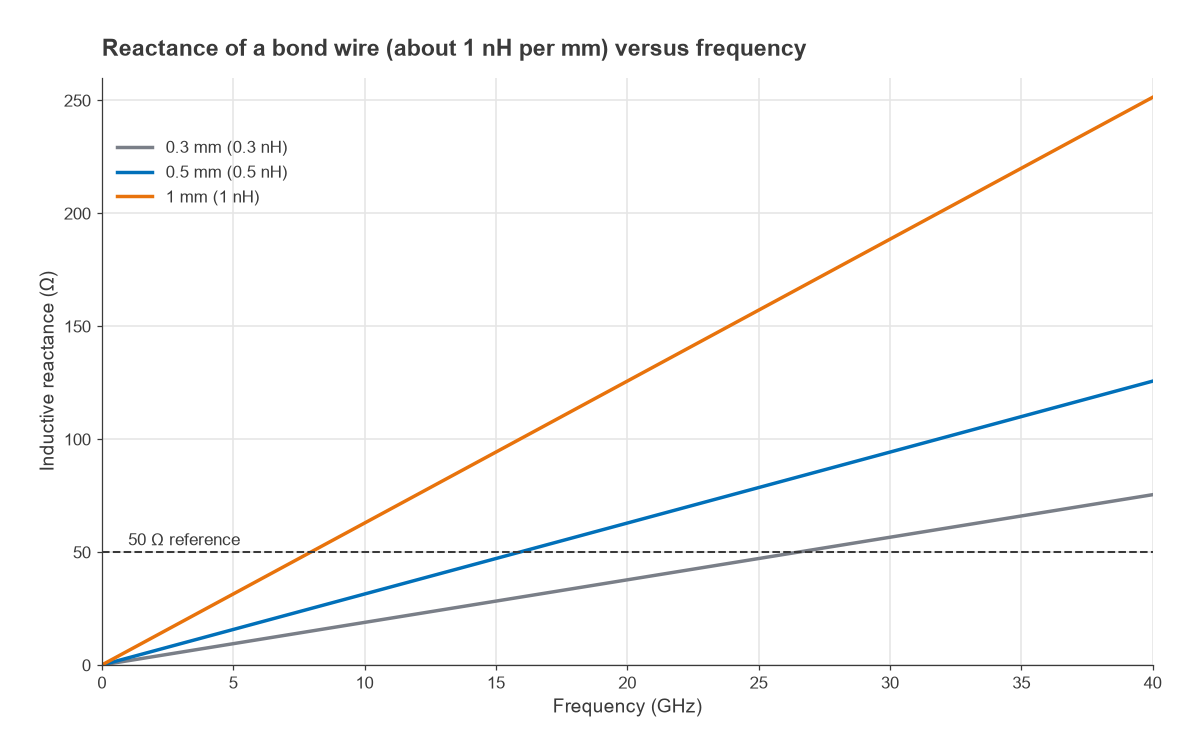
- A 0.5 mm wire (about 0.5 nH) has 7.5 Ω of reactance at 2.4 GHz, small enough to absorb into a matching network.
- At 10 GHz the same wire has 31.4 Ω, and at 30 GHz it has 94.2 Ω, almost twice the 50 Ω system impedance.
- The wire reaches 50 Ω at 15.9 GHz. A 1 mm wire reaches it at 8.0 GHz and a 0.3 mm wire at 26.5 GHz.
Package leads, pads and solder joints add similar parasitics, as described in RF component parasitics. Below a few gigahertz they are manageable and discrete design works well. Above roughly 10 to 20 GHz they start to dominate, and keeping the matching network on the same die as the transistor becomes the only practical way to control it. That is the main reason microwave and millimetre-wave radio front-ends use MMICs or RFICs rather than discrete transistors. Where interconnect cannot be avoided, flip-chip mounting or short ribbon bonds reduce the inductance, and EM simulation of the transition becomes part of the design.
Cost Structure
Integrated circuits trade high fixed cost for low unit cost. Mask sets, design tools, multi-project wafer runs and the engineering effort of a tape-out are paid once, and each fabrication cycle typically takes weeks to months. Discrete design has almost no fixed cost, but the unit cost includes every part, the assembly and the board area, and it does not fall much with volume.
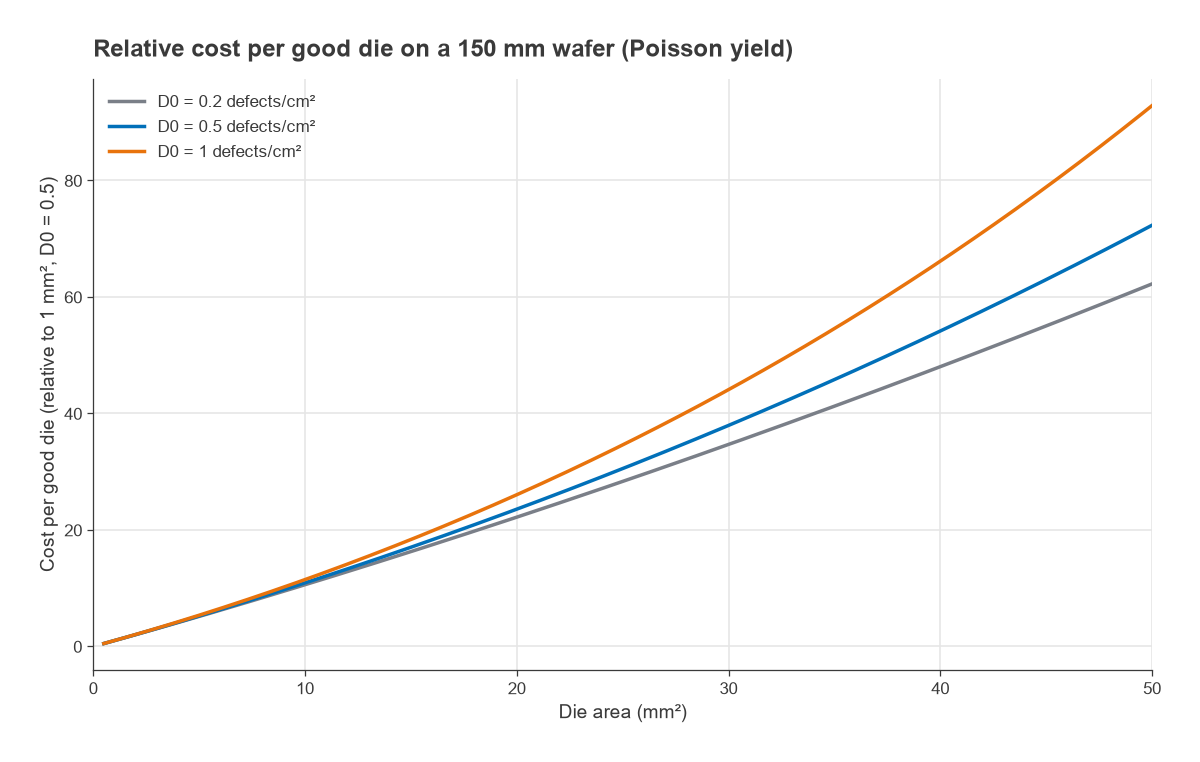
Once a chip is in production, its cost is roughly the wafer cost divided by the number of good dies. The number of gross dies on a round wafer of diameter d is approximately
DPW ≈ π(d/2)2/A − πd/√(2A)
where A is the die area and the second term accounts for partial dies at the edge. A simple Poisson model gives the fraction of dies free of random defects as Y = exp(−D0A), with D0 the defect density.
Worked example: die area and cost per good die
Take a 150 mm wafer, a common diameter for compound semiconductor processes, and an assumed defect density of 0.5 per cm2.
- A 4 mm2 die: DPW ≈ 17,671/4 − 471.2/2.83 = 4,251 gross dies. Y = exp(−0.5 × 0.04) = 98.0 %, so about 4,167 good dies.
- A 25 mm2 die: DPW ≈ 706.9 − 66.6 = 640 gross dies. Y = exp(−0.5 × 0.25) = 88.3 %, so about 565 good dies.
- The larger die is 6.25 times the area but costs about 7.4 times as much per good die, because both the edge loss and the yield get worse.
The lesson for MMIC design is that area is cost. Spiral inductors and quarter-wave lines are large at low frequency, so a 2 GHz MMIC spends most of its die on passives. At 30 GHz the same functions shrink by more than ten times, which is part of why MMICs become more economical as frequency rises. In silicon RFICs the wafer is cheaper per unit area and larger (300 mm is common), but a complete transceiver die is also much larger.
MMIC vs RFIC vs Discrete Comparison
| Factor | Discrete | MMIC | RFIC |
|---|---|---|---|
| Typical process | Any packaged transistor | GaAs, GaN, InP, sometimes SiGe | CMOS, SOI, SiGe BiCMOS |
| Frequency sweet spot | Up to a few GHz, higher with care | Microwave and mmWave | Sub-GHz to mmWave, set by process node |
| Output power | Highest with large packaged devices | High with GaN | Low to moderate |
| Noise figure | Best with selected low-noise devices | Very good | Good, limited by on-chip passives |
| Fixed cost and lead time | Lowest, days to weeks | High, months per spin | Highest, months per spin |
| Unit cost at high volume | Moderate, falls slowly | Low to moderate | Lowest per function |
| Tunability after build | Full | Limited to external parts | Digital trims and calibration |
| Size | Largest | Small | Smallest per function |
When to Use Discrete Design
Discrete design remains the right choice more often than its reputation suggests.
- Low volume or one-off systems, where tape-out cost cannot be recovered. Test equipment, scientific instruments and many defence and space programmes fall here.
- Best possible noise figure at low microwave frequencies. A selected discrete HEMT with a high-Q off-chip input match can beat an integrated LNA, which is why many front-ends for radio astronomy and satellite ground stations stay discrete. See the LNA design article.
- High power at HF to low microwave, where large packaged transistors and lumped matching outperform anything that fits on a die. Output networks for power amplifier classes such as E or F often need high-Q harmonic terminations that are easier to build off-chip.
- Unusual or changing requirements, where the ability to retune on the bench outweighs size.
In practice most products mix all three. A typical radio uses an RFIC transceiver, MMIC or module power amplifiers and switches, and a handful of discrete parts for filtering, matching and protection. The RF front-end modules article shows how those pieces are packaged together, and the board-level side is covered in RF PCB layout.
Frequently Asked Questions
What is an MMIC?
An MMIC is a monolithic microwave integrated circuit: one die holding the transistors, matching networks and bias elements of a complete microwave function. Most are made on GaAs, GaN or InP and have 50 Ω RF ports so they can be dropped into a system with little external matching.
Is an MMIC the same as an RFIC?
The terms overlap, and some engineers use them interchangeably. In common usage, MMIC suggests a compound-semiconductor die with one RF function, while RFIC suggests a silicon chip combining RF with mixed-signal and digital circuits.
Why are MMICs used at millimetre-wave frequencies?
At those frequencies package leads and bond wires have reactances comparable to or larger than 50 Ω, so matching networks have to sit on the die right next to the transistor. Passive elements also become small enough to fit economically on chip.
Can CMOS replace GaAs?
For many receive and low-power transmit functions it already has, especially where digital calibration can correct analog errors. GaAs and GaN keep their place where output power, breakdown voltage, noise or passive Q matter more than integration.
Related Topics
The RFIC design hub introduces on-chip design methods. Related reading includes MIMO, beamforming and phased arrays, where highly integrated beamformer ICs are common, broadband RF amplifier design, and harmonic balance simulation for verifying nonlinear MMIC and RFIC blocks before tape-out.