

Electromagnetic interference (EMI) is unwanted electromagnetic energy that disturbs the operation of a circuit or system. Electromagnetic compatibility (EMC) is the property of a device that neither emits enough of that energy to disturb other equipment nor is itself disturbed by the energy it encounters. EMI is the problem; EMC is the design goal and the set of tests that prove it has been met.
For an RF designer, EMC is partly familiar ground: the same physics that makes an antenna radiate makes a cable or a ground loop radiate. The difference is that EMC concerns energy at frequencies and in places where nobody intended it. This page sits under RF PCB layout in the RF design guide and covers radiated and conducted emissions, the differential- and common-mode mechanisms behind them, the field equations used for estimates, and how pre-compliance measurements are set up and read.
EMC vs EMI: Definitions
EMI describes an effect: a disturbance coupled from a source to a victim through some path. Every fix removes or weakens one of the three. EMC describes a state in which the source, path and victim have been arranged so that no disturbance occurs in the intended environment. Regulators turn that state into measurable limits.
The coupling path can be conducted, along power, signal or ground wires, or radiated, through near-field capacitive and inductive coupling or far-field radiation. Below roughly 30 MHz, cables are short compared with a wavelength and are poor radiators, so standards measure conducted noise on mains leads. Above about 30 MHz, radiation dominates and the tests switch to field strength measured with an antenna.
Emissions and Immunity
EMC testing splits into two halves. Emissions tests measure what the equipment under test (EUT) produces: radiated field strength and conducted voltage or current on cables. Immunity, or susceptibility, tests expose the EUT to disturbances and check that it keeps working: radiated RF fields, conducted RF injected onto cables, electrostatic discharge, fast transients, surges and supply dips. Typical radiated immunity levels for commercial products are a few volts per metre, with higher levels for industrial and automotive environments; the exact figures depend on the product standard.
Intentional radiators add a third category. A radio transmitter must meet limits on spurious emissions, harmonics and out-of-band power under radio regulations as well as the general EMC rules for its digital circuitry.
Radiated Emissions
Two simple models explain most radiated emission problems: the small current loop formed by a signal and its return, and the short wire or cable carrying a current that has no nearby return. They correspond to differential-mode and common-mode current.
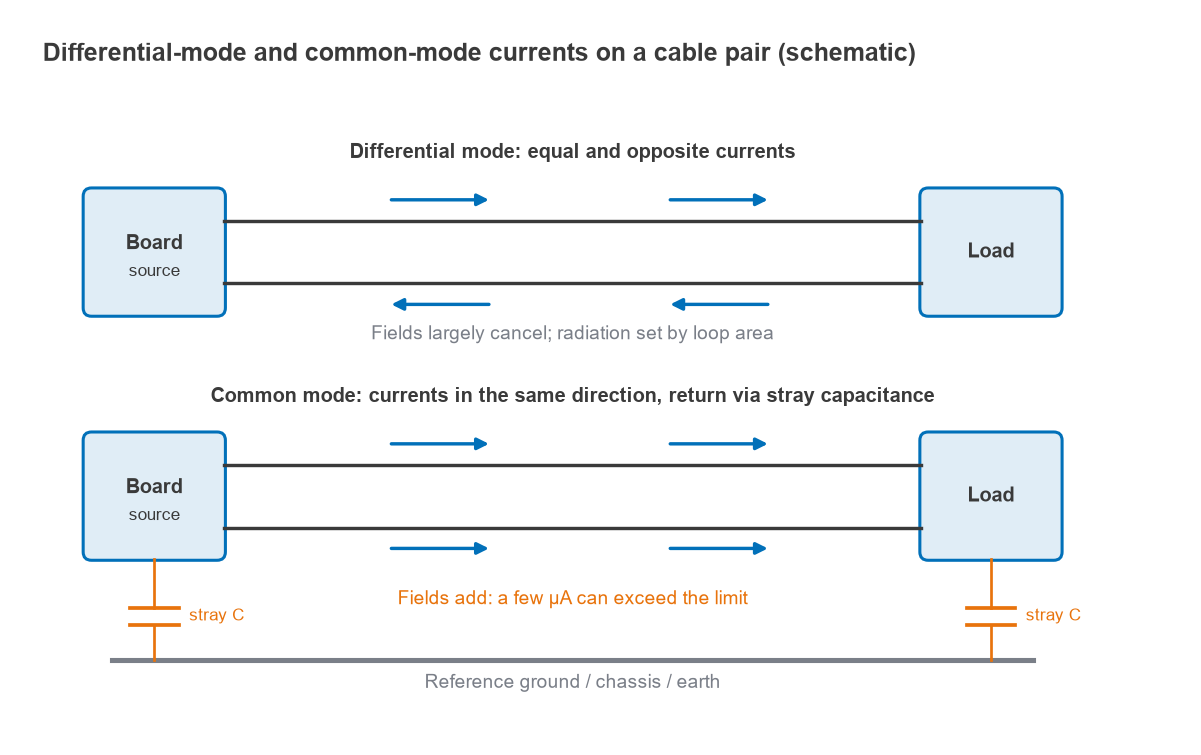
Differential-mode radiation
Differential-mode current flows out along a trace and back along its return path. The two currents are equal and opposite, so their fields largely cancel, and what remains behaves like a small loop antenna. For a loop of area A (m2) carrying current I (A) at frequency f (Hz), the maximum far-field strength at distance r (m) in free space is approximately
E ≈ 1.316 × 10⁻¹⁴ · f2 · A · I / r (V/m)
The f2 term means differential-mode emission rises 40 dB per decade of frequency for a constant current. Over a reflecting ground plane, as on an open-area test site, the reflected wave can add up to 6 dB. The controls are loop area, which layout sets, and the current spectrum, which edge rates and filtering set.
Common-mode radiation
Common-mode current flows in the same direction on all conductors of a cable and returns through stray capacitance to the surroundings. There is no nearby return to cancel its field, so the cable acts as a monopole or dipole antenna. For a cable of length L that is short compared with a wavelength, the field is approximately
E ≈ 1.257 × 10⁻⁶ · f · L · I / r (V/m)
This rises only 20 dB per decade, but the coefficient is enormous compared with the loop formula. Common-mode current arises from ground-potential differences across a board, from imbalance in a nominally differential pair, and from return current forced around a gap in a reference plane. A pair with skew or unequal loading converts differential signals to common mode; the quantity that describes this is Scd21 in mixed-mode S-parameters.
Worked example: loop versus cable
Compare the two mechanisms at a 3 m test distance against an approximate Class B limit. Commonly quoted FCC Class B radiated limits at 3 m are about 40 dBµV/m from 30 to 88 MHz and 43.5 dBµV/m from 88 to 216 MHz; check the current rules for any real product.
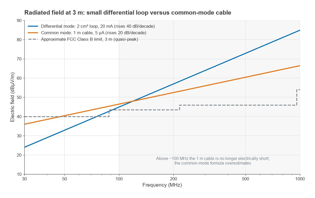
- Differential mode: a 20 mA harmonic at 100 MHz in a loop of 2 cm2 (2 × 10⁻⁴ m2). E = 1.316 × 10−14 × (108)2 × 2 × 10−4 × 0.02 / 3 = 175 µV/m, or 20·log(175) = 44.9 dBµV/m. That is about 1.4 dB over the 43.5 dBµV/m line. Halving the loop area gains 6 dB; reaching 40 dBµV/m needs the loop shrunk to 1.14 cm2.
- Common mode: 5 µA on a 1 m cable at 30 MHz, where the cable is λ/10 and still reasonably short. E = 1.257 × 10−6 × 3 × 107 × 1 × 5 × 10−6 / 3 = 62.9 µV/m, or 36.0 dBµV/m. The current that would reach the 40 dBµV/m limit is 8.0 µA.
Microamps of common-mode current on a cable produce the same field as tens of milliamps in a small loop. That is why a clamp-on current probe on each cable is one of the most useful pre-compliance tools. Above about 100 MHz a 1 m cable is no longer electrically short, and the simple formula overestimates the field; the cable then behaves as a resonant antenna and peaks near its quarter- and half-wave resonances.
Conducted Emissions
Conducted emissions tests measure the RF voltage that the EUT puts back onto its mains or DC supply leads, typically from 150 kHz to 30 MHz. A line impedance stabilisation network (LISN) is inserted between the supply and the EUT. It presents a defined impedance, commonly 50 Ω in parallel with 50 µH, to the EUT across the band, blocks noise from the supply, and provides a 50 Ω port for the receiver or spectrum analyser.
Limits are expressed in dBµV. In a 50 Ω system, dBµV = dBm + 107, so 1 mV is 60 dBµV and −47 dBm. Commonly quoted Class B quasi-peak limits for multimedia and IT equipment are around 66 dBµV falling to 56 dBµV over 150 to 500 kHz, 56 dBµV from 0.5 to 5 MHz and 60 dBµV from 5 to 30 MHz, with average-detector limits about 10 dB lower; treat these as approximate. Switching regulators are the usual source, with differential-mode noise from ripple current and common-mode noise from the fast switch node coupling through heatsink and transformer capacitance. See also RF power supply decoupling.
Why RF Designs Have Particular EMC Problems
- High-level local oscillators and their harmonics can leak through the antenna port, through gaps in a shield, or along supply and control lines.
- Power amplifier harmonics and wideband noise must sit below spurious emission limits that are often far tighter than general EMC limits.
- Sensitive receivers are their own victims: a clock harmonic that easily passes a regulatory limit can still desensitise an LNA on the same board, a problem treated in RF coexistence.
- Strong transmitted fields from the product’s own antenna can couple into audio, sensor and supply circuits, which can then malfunction during normal operation, an immunity problem the product creates for itself.
Design Techniques for EMC
Most EMC design is about controlling return current. A continuous reference plane under every high-speed or RF trace keeps the return directly beneath the signal, which minimises loop area and keeps the ground at one potential. Gaps and splits in that plane force the return current around them, creating both a larger loop and a voltage across the gap that drives common-mode current onto anything connected on either side. Via fences and stitching along plane edges, covered in RF grounding and via stitching, limit edge radiation and cavity resonances.
At the board edge, every cable is a potential antenna. Filtering each line where it leaves the board, with the filter’s ground tied directly to the chassis or plane at the connector, stops noise before it reaches the cable. Common-mode chokes and ferrites raise the impedance to common-mode current while passing differential signals. Balanced interfaces and baluns help only as far as their balance holds at the frequencies of concern. Metal enclosures and board-level cans, discussed in RF shielding, block radiated coupling, but apertures and seams must be small compared with a wavelength, and any cable that passes through a shield without filtering carries the noise straight out.
At the source, slower edges, spread-spectrum clocking and careful decoupling reduce the current spectrum. Stackup also matters; see FR-4 versus Rogers.
Pre-Compliance Testing
Formal compliance testing takes place in an accredited laboratory with a semi-anechoic chamber or open-area test site, calibrated antennas, a CISPR receiver and specified detectors. Pre-compliance testing uses simpler equipment on the bench to find and fix problems before that visit. A spectrum analyser with a peak detector, a LISN, near-field probes, a current clamp and an inexpensive antenna cover most needs.
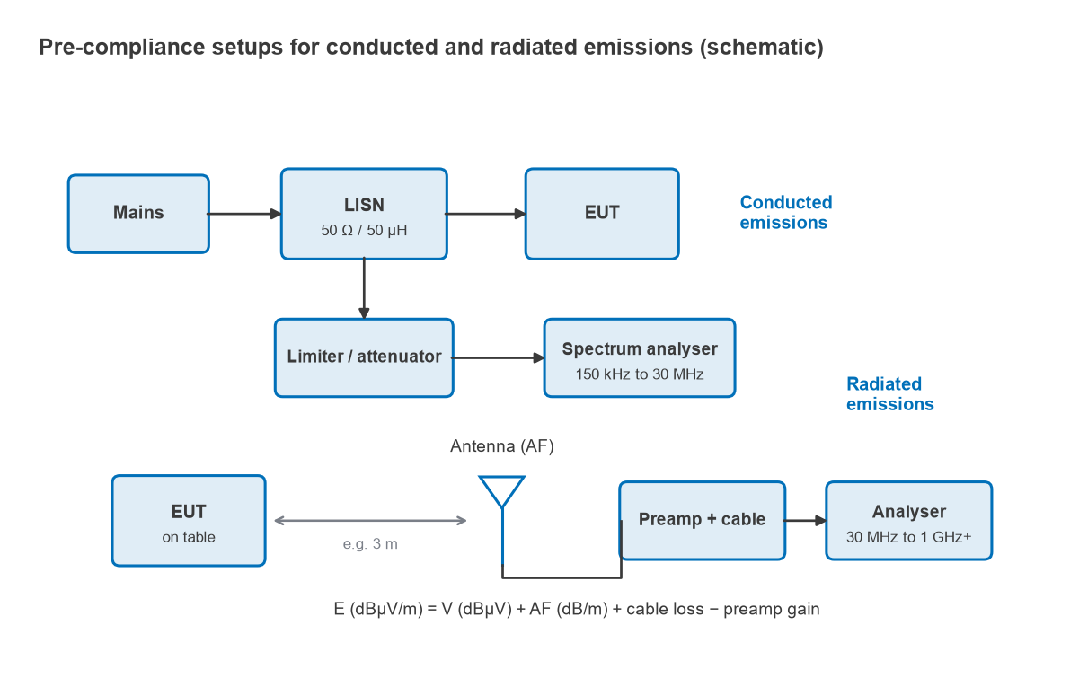
The receiver bandwidths commonly specified are 9 kHz from 150 kHz to 30 MHz and 120 kHz from 30 MHz to 1 GHz. A peak detector always reads at or above quasi-peak and average, so a peak scan that passes the quasi-peak limit is a safe result, while a peak reading above the limit needs a quasi-peak measurement to settle the question.
Converting an analyser reading to field strength
The antenna factor (AF, in dB/m) converts the voltage at the antenna terminals to the incident field:
E (dBµV/m) = V (dBµV) + AF (dB/m) + cable loss (dB) − preamplifier gain (dB)
For example, an analyser reading of 25 dBµV with an antenna factor of 18 dB/m at that frequency and 2 dB of cable loss gives E = 25 + 18 + 2 = 45 dBµV/m. Against a 43.5 dBµV/m limit this emission fails by 1.5 dB. Because bench setups are not calibrated sites and reflections can shift readings by several dB, many teams treat a pre-compliance margin of several dB below the limit as the target before booking a laboratory.
Near-field probes do not give absolute field strengths, but they find sources quickly. An H-field loop held over a board shows which trace, regulator or connector carries the current at the offending frequency, and an E-field probe shows which areas carry high voltage. More on measurement methods is in Radio Architectures Part 20: measuring radio performance.
Frequently Asked Questions
What is the difference between EMC and EMI?
EMI is the unwanted disturbance itself, coupled from a source to a victim. EMC is the ability of equipment to work in its environment without causing or suffering that disturbance, demonstrated by emissions and immunity tests.
Why is common-mode current so important?
Common-mode current on a cable has no nearby return to cancel its field, so the cable radiates like an antenna. A few microamps can produce as much field as tens of milliamps of differential-mode current in a small loop.
What is the difference between radiated and conducted emissions?
Conducted emissions are RF voltages on supply cables, measured through a LISN, usually from 150 kHz to 30 MHz. Radiated emissions are fields measured with an antenna at a set distance, usually from 30 MHz upward.
Is pre-compliance testing worth doing?
Yes, because it finds the dominant sources early, when layout and filtering changes are cheap. Its readings are not absolute, so it is best used to compare designs and to establish a margin rather than to claim a pass.
Related Topics
The RF PCB layout hub covers stackup, grounding, shielding and decoupling, all of which shape EMC performance. For the measurement side, see RF measurement and test, and for unit conversions such as dBm to dBµV see dB and dBm explained.