

Resolution bandwidth (RBW) is the bandwidth of the final IF filter in a spectrum analyzer, and it sets how closely spaced two signals can be and still appear as separate peaks. A spectrum analyzer is a frequency-selective receiver that displays power against frequency. Narrowing the RBW separates close signals and lowers the displayed noise floor, at the cost of a slower sweep.
Harmonics, spurs, adjacent-channel power and phase noise are all measured on a spectrum analyzer, and a careless setting can hide a weak signal under the noise floor or create intermodulation inside the analyzer that looks like a defect in the device under test. This page explains the swept superheterodyne architecture, the three settings that matter most (RBW, VBW and input attenuation), and a short procedure for measuring low-level signals. It belongs to the RF measurement section of the RF design reference.
How a swept spectrum analyzer works
A traditional spectrum analyzer is a superheterodyne receiver whose local oscillator is swept. The input signal passes through a step attenuator and a low-pass or tracking preselector filter, then reaches the first mixer. The LO is tuned by a ramp, so at each instant only the input frequency that converts to the fixed IF passes the IF filter. A logarithmic amplifier and an envelope detector turn that IF power into a voltage, a video filter smooths it, and the result is plotted against the same ramp that tunes the LO. The display is therefore a record of power through a narrow filter as the filter is dragged across the band.
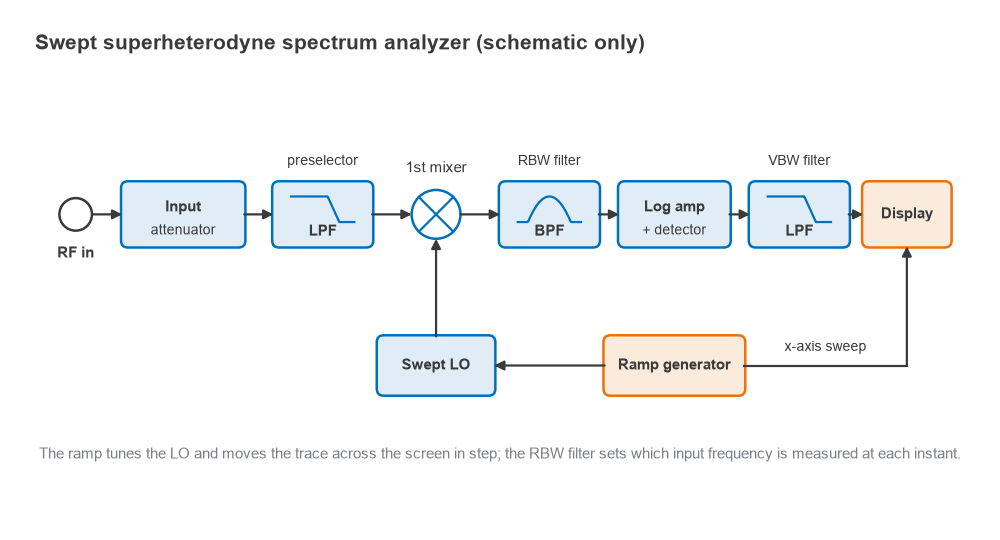
The architecture is the same one described for receivers in Radio Architectures Part 2, with the same weaknesses: image responses, LO feedthrough and mixer nonlinearity. Most microwave analyzers use a high first IF so that the image falls far above the input range, followed by one or two further conversions to a low final IF where the RBW filters are built. Modern instruments digitize that final IF and implement the RBW filter, detector and video filter in DSP, and some compute an FFT over a captured block instead of sweeping, but the controls and the noise and distortion arguments below are unchanged.
Resolution bandwidth (RBW)
The RBW filter decides what the analyzer can resolve. A pure tone does not appear as a vertical line but as a copy of the RBW filter shape, traced out as the filter sweeps past it. Two equal tones are resolved when their spacing is at least about one RBW. When their levels differ, the filter skirts matter, which analyzers specify as shape factor, the ratio of the 60 dB bandwidth to the 3 dB bandwidth. Gaussian-like analog filters typically have a shape factor between about 4 and 15, and digital RBW filters can be much sharper.
RBW also sets how much noise reaches the detector. The analyzer’s own noise is spread evenly across frequency, so the displayed noise power is proportional to RBW. Reducing RBW by a factor of 10 lowers the noise floor by 10 dB, while a CW tone keeps the same displayed level because all of its power still fits inside the filter.
The price is speed. A filter of bandwidth RBW needs a settling time of roughly 1/RBW, and the sweep must move slowly enough that the filter has that long to respond as it crosses a signal. For a swept analog filter this gives the approximate relation
tsweep ≈ k × Span / RBW2
with k typically between 2 and 3. With k = 2.5 and a 10 MHz span, RBW = 100 kHz gives a 2.5 ms sweep, RBW = 10 kHz gives 0.25 s and RBW = 1 kHz gives 25 s.
Video bandwidth (VBW) and detectors
The video filter is a low-pass filter after the detector. It does not change resolution or the average noise level; it smooths the trace, so a small signal just above the noise becomes easier to see. Common practice is VBW equal to RBW, or up to three times RBW, for signal measurements, and VBW of 0.1 × RBW or less when the goal is a smooth noise floor. Narrowing VBW below RBW also lengthens the sweep, because the video filter now has the longer settling time.
The detector decides which value represents each display point. Peak detection never misses a narrow signal and suits spur searches; average (RMS) detection reports true power and suits noise-like modulated signals and channel-power or ACLR measurements. Averaging the logarithm of noise, rather than its power, reads about 2.5 dB low, so noise measured in log-average mode needs that correction or an RMS detector.
Displayed average noise level (DANL)
DANL is the analyzer’s own noise floor as it appears on screen with no signal applied and the input terminated. It follows from the same thermal noise kTB calculation used for any receiver:
DANL (dBm) ≈ −174 dBm/Hz + NFSA + 10log(RBW) + attenuation
where NFSA is the analyzer’s noise figure with 0 dB input attenuation, and small detector corrections are ignored. General-purpose analyzers without a preamplifier commonly have noise figures in the twenties of dB, which is far worse than a receiver front end; an internal preamplifier can bring that down substantially. Data sheets often quote DANL normalized to a 1 Hz RBW.
Worked example: finding a −125 dBm tone
Take an analyzer with a 24 dB noise figure and 0 dB input attenuation. At RBW = 10 kHz the DANL is −174 + 24 + 40 = −110 dBm. At 1 kHz it is −120 dBm, and at 100 Hz it is −130 dBm. A −125 dBm tone is invisible at the first two settings and stands 5 dB above the noise at the third. Setting the attenuator to 10 dB instead of 0 dB raises every one of those floors by 10 dB, so the 1 kHz floor moves from −120 dBm to −110 dBm.
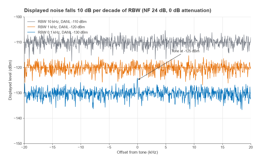
A signal close to the noise floor also reads high, because the analyzer displays signal plus noise. A tone exactly at the noise level reads about 3.0 dB high, one 6 dB above it reads about 1.0 dB high, and one 10 dB above it reads about 0.4 dB high. A signal-to-noise ratio of 10 dB or more is therefore a sensible minimum for amplitude measurements.
The input attenuator and mixer level
The input attenuator sets the mixer level, which is the input power minus the attenuation. Too high a mixer level creates harmonics and intermodulation; too low a level wastes dynamic range, since every decibel of attenuation adds a decibel to DANL. The attenuator also protects the mixer: most analyzers specify a maximum safe input in the region of +30 dBm with attenuation in circuit, and much less with 0 dB attenuation.
The analyzer’s first mixer behaves like any other nonlinear stage. Its distortion can be described by a third-order intercept (TOI) and a second-harmonic intercept (SHI), referred to the mixer input, exactly as in intermodulation and intercept points. For two equal tones at mixer level Pmix, the third-order products sit at
IM3 (dBc) = −2 × (TOI − Pmix)
and a single tone produces a second harmonic at −(SHI − Pmix) dBc. Noise relative to the signal is DANL − Pmix, which improves by 1 dB for each decibel of extra mixer level, while IM3 worsens by 2 dB and the second harmonic by 1 dB.
The dynamic range chart
Plotting those three lines against mixer level gives the dynamic range chart. The best mixer level for third-order measurements is where the noise line and the IM3 line cross:
Popt = (DANL + 2 × TOI) / 3, and the distortion-free range is (2/3) × (TOI − DANL).
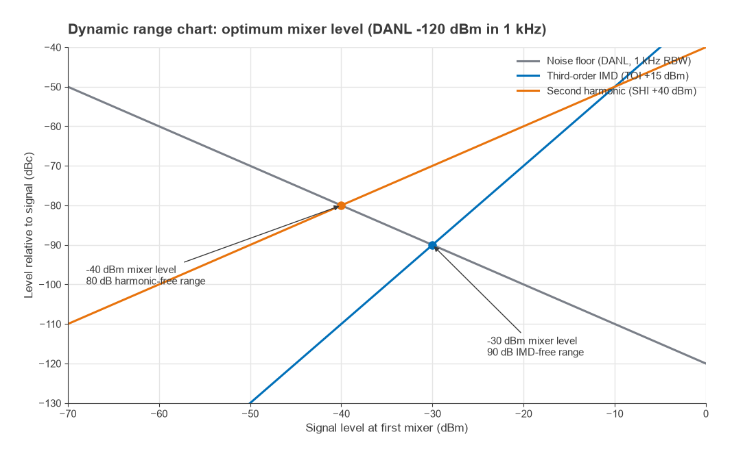
With an illustrative TOI of +15 dBm and DANL of −120 dBm in a 1 kHz RBW, Popt = (−120 + 30)/3 = −30 dBm and the range is (2/3) × 135 = 90 dB. For second harmonics with an SHI of +40 dBm the optimum is (−120 + 40)/2 = −40 dBm and the range is 80 dB. Narrowing RBW lowers the noise line and moves both optima to lower mixer levels. The same reasoning appears for receivers in SFDR and dynamic range.
Avoiding analyzer-generated intermodulation
A two-tone test is only useful if the IM3 products on screen come from the device and not the analyzer. Consider two tones at −10 dBm each at the analyzer input, with 10 dB attenuation. The mixer level is −20 dBm, so with TOI = +15 dBm the analyzer creates its own IM3 at −2 × (15 − (−20)) = −70 dBc, or −80 dBm referred to the input. If the device’s true IM3 is near −80 dBm, the reading could be wrong by several decibels either way, since the two contributions add with unknown phase.
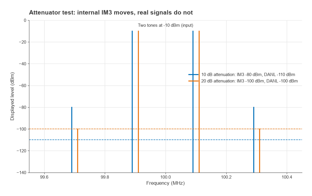
The attenuator test exposes the problem. Increase the attenuation by 10 dB. The analyzer corrects its display for the attenuator, so real signals stay at the same displayed level. Internally generated third-order products fall by 20 dB relative to the tones, in this example from −80 dBm to −100 dBm, while the noise floor rises by 10 dB. If the IM3 reading does not move when the attenuation changes, the products are real. If it drops, the analyzer was contributing.
When measuring a weak harmonic next to a strong fundamental, a high-pass or notch filter ahead of the analyzer keeps the fundamental away from the mixer. Strong carriers outside the displayed span also reach the first mixer unless a preselector removes them.
How to measure low-level signals
A practical sequence for finding and measuring a weak signal:
- Check the total power at the input, including signals outside the span, and confirm it is within the safe limit for the attenuation you intend to use.
- Reduce the input attenuation, in steps, toward 0 dB. Each 10 dB removed lowers DANL by 10 dB, provided the mixer stays well below compression.
- Narrow the span around the signal, then reduce RBW. Each decade of RBW reduction lowers the floor by 10 dB.
- Turn on the internal preamplifier if fitted, or add an external low-noise amplifier ahead of the analyzer, accounting for its gain.
- Reduce VBW or use trace averaging to smooth the noise so the signal stands out.
- Correct for signal-plus-noise if the signal is within 10 dB of the floor, and use a noise marker (normalized to 1 Hz with an RMS detector) when the quantity of interest is a noise density.
Noise density measurements made this way are the basis of the Y-factor and cold-source methods in noise figure measurement and of direct-spectrum phase noise measurement. Whole-radio tests that combine several of these settings are described in Measuring Radio Performance.
Frequently asked questions
What is RBW?
RBW is the bandwidth of the spectrum analyzer’s final IF filter. It sets the smallest frequency spacing at which two signals appear as separate peaks, and it sets the displayed noise floor, which changes by 10 dB per decade of RBW. Narrow RBW gives better resolution and sensitivity but slower sweeps.
How do you measure low-level signals?
Lower the input attenuation, narrow the span and RBW, enable a preamplifier and smooth the trace with VBW or averaging. Each step lowers or steadies the noise floor. Check that strong signals at the input do not overload the mixer once the attenuation is reduced.
How can you tell if intermodulation is coming from the analyzer?
Change the input attenuation by 10 dB and watch the products. Real signals keep the same displayed level. Third-order products made inside the analyzer change by about 20 dB relative to the tones, and second-order products by about 10 dB.
Related topics
The companion instrument for linear measurements is covered in VNA basics, and short definitions of RBW, DANL and related terms are in the wireless terms glossary.