

RF connectors are coaxial interfaces that join cables, components and instruments while keeping a controlled impedance, usually 50 Ω, up to a stated maximum frequency. The main types are BNC and F for low-frequency and video use, Type N and TNC for rugged outdoor work, SMA for general use to 18 GHz, and the precision 3.5 mm, 2.92 mm, 2.4 mm, 1.85 mm and 1.0 mm families for millimetre-wave test.
A connector is a short piece of coaxial transmission line with a mechanical coupling. It must match the line’s impedance, keep its dimensions repeatable across hundreds of connections, and stay free of higher-order modes up to its rated frequency. Pick the wrong one and the reflection, loss or poor repeatability shows up directly in the measured VSWR and return loss. This page compares the common connector families on frequency limit, impedance and coupling torque, explains where the frequency limit comes from, and covers cable selection. It belongs to the RF passive components section of the RF design reference.
Impedance and the coaxial geometry
The characteristic impedance of a coaxial line depends only on the ratio of the outer conductor’s inner diameter D to the centre conductor diameter d, and on the dielectric constant εr:
Z0 = (60 / √εr) × ln(D / d)
Most RF work uses 50 Ω, a compromise between the lowest loss (near 77 Ω for an air line) and the highest power handling (near 30 Ω). Video, cable TV and some broadcast systems use 75 Ω. The two are not interchangeable: 75 Ω BNC and Type N connectors look like their 50 Ω versions but have different centre pin sizes, and mating them can damage the female contact or create a mismatch. With Z0 mismatched by 50 to 75 Ω, the reflection coefficient is (75 − 50)/(75 + 50) = 0.2, a return loss of only 14 dB. The background is in types of transmission lines.
Why each connector has a frequency limit
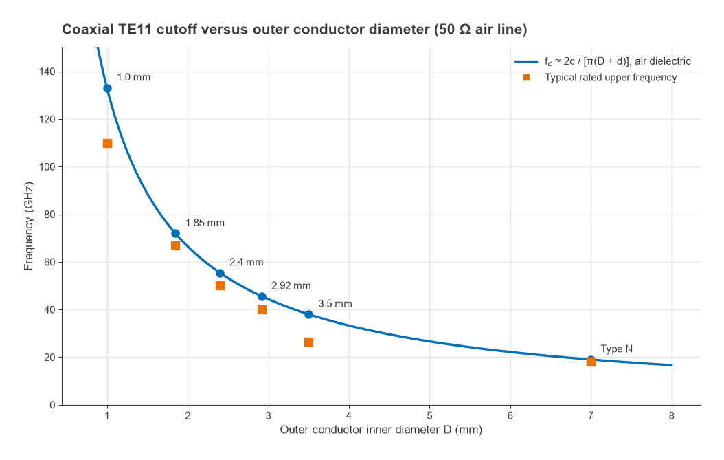
A coaxial line carries only the TEM mode until the first waveguide mode, TE11, can propagate. Its cutoff is approximately
fc ≈ 2c / [π (D + d) √εr]
Above fc, energy can convert into the TE11 mode at any discontinuity, producing sharp resonances and unpredictable loss. The only way to raise the limit is to shrink the line, which is why the precision connectors are named after their outer conductor diameter.
Worked example: cutoff of common interfaces
- Type N: D = 7.00 mm, d = 3.04 mm, air. Z0 = 60 ln(2.30) = 50.0 Ω, and fc = 2 × 3 × 108 / (π × 10.04 mm) = 19.0 GHz. Precision Type N is rated to 18 GHz, just below this.
- SMA: PTFE-filled, D ≈ 4.13 mm, d ≈ 1.27 mm, εr ≈ 2.05. Z0 = 49.4 Ω and fc ≈ 24.7 GHz, which is why good SMA parts can be used to about 26.5 GHz, while 18 GHz is the common rating.
- 3.5 mm: air line, D = 3.50 mm, d = 1.52 mm, fc = 38.0 GHz. Support beads lower the practical limit to about 34 GHz.
- 2.92 mm: fc = 45.5 GHz. 2.4 mm: 55.4 GHz. 1.85 mm: 71.9 GHz. 1.0 mm: 133 GHz.
In each case the rated frequency sits somewhat below the ideal cutoff, leaving margin for bead discontinuities, tolerances and the slot and finger structure of the female contact.
Connector comparison table
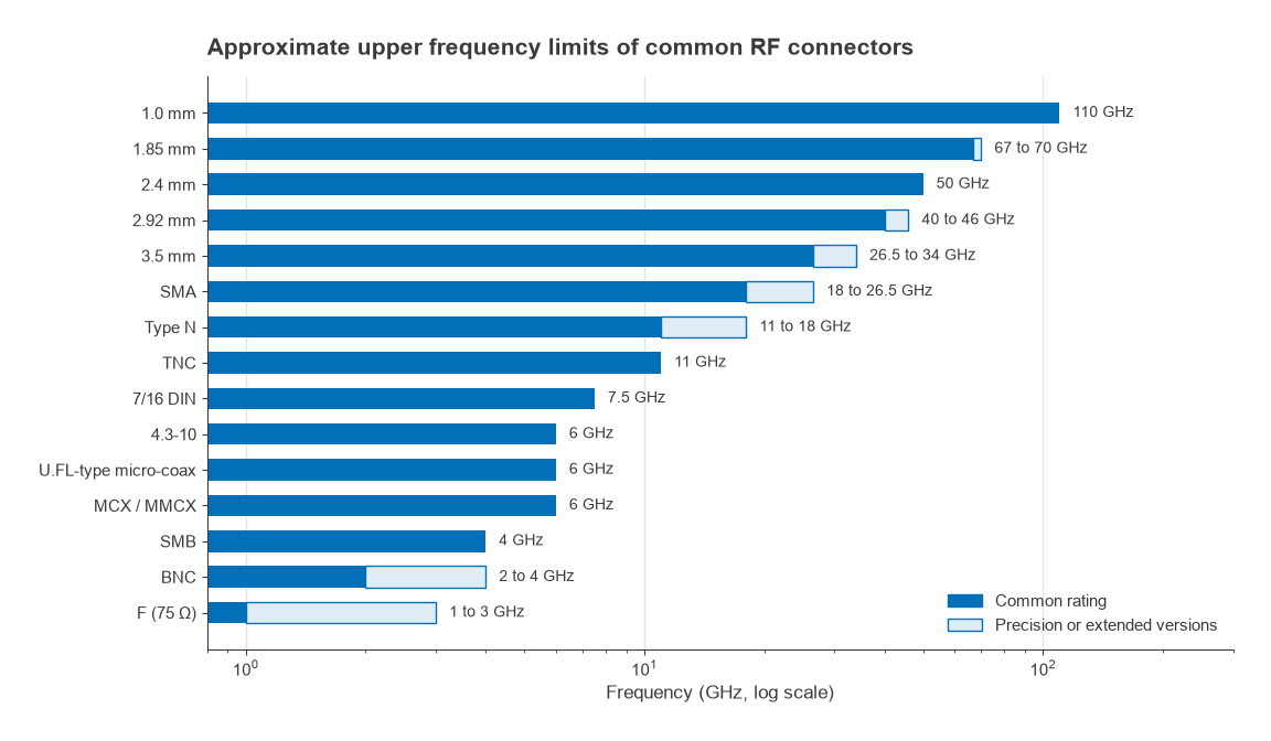
Frequency limits and torques are typical approximate values as of 2026. The connector manufacturer’s data sheet, or the relevant interface standard, takes precedence for any specific part.
| Connector | Impedance | Approx. upper frequency | Coupling | Typical torque | Typical use |
|---|---|---|---|---|---|
| BNC | 50 Ω or 75 Ω | About 2 to 4 GHz | Bayonet | None (bayonet) | Lab instruments, video, low-frequency test |
| F | 75 Ω | About 1 to 3 GHz | Threaded | Hand tight | Cable TV, satellite TV |
| SMB, MCX, MMCX | 50 Ω | About 4 to 6 GHz | Snap-on | None | Internal board-to-cable links |
| U.FL-type micro-coaxial | 50 Ω | About 6 GHz | Snap-on | None; limited mating cycles | Antenna links inside wireless modules |
| TNC | 50 Ω | About 11 GHz | Threaded BNC | Per manufacturer | Vibration-prone and outdoor equipment |
| Type N | 50 Ω (75 Ω version exists) | 11 GHz standard, 18 GHz precision | Threaded | About 1.36 N·m (12 in-lb) | Outdoor, antennas, higher power, test |
| 7/16 DIN, 4.3-10 | 50 Ω | About 7.5 GHz and 6 GHz | Threaded (4.3-10 also push-pull) | About 25 to 30 N·m for 7/16 DIN; about 5 N·m for screw-type 4.3-10 | Base station feeders, low PIM |
| SMA | 50 Ω | 18 GHz common, up to about 26.5 GHz | Threaded | About 0.56 N·m (5 in-lb) brass, 0.9 N·m (8 in-lb) stainless | General RF modules and boards |
| 3.5 mm | 50 Ω | 26.5 GHz, mode-free to about 34 GHz | Threaded | About 0.9 N·m (8 in-lb) | Test ports and calibration kits |
| 2.92 mm | 50 Ω | 40 GHz, some to about 46 GHz | Threaded | About 0.9 N·m (8 in-lb) | Millimetre-wave modules and test |
| 2.4 mm | 50 Ω | 50 GHz | Threaded | About 0.9 N·m (8 in-lb) | 50 GHz test equipment |
| 1.85 mm | 50 Ω | 67 GHz, some to about 70 GHz | Threaded | About 0.9 N·m (8 in-lb) | 67 GHz test equipment |
| 1.0 mm | 50 Ω | About 110 GHz | Threaded | Lower, per manufacturer | W-band test |
Torque, intermating and care
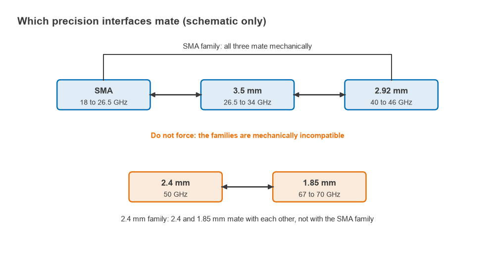
Threaded connectors are repeatable only when tightened to a consistent torque with a calibrated wrench, turning the nut and never the connector body. Over-tightening deforms the contacts and reference planes; under-tightening leaves a variable gap. SMA, 3.5 mm and 2.92 mm interfaces mate mechanically with each other, which is convenient but risky: an SMA with a poorly controlled pin depth or a damaged dielectric face can damage a precision 3.5 mm or 2.92 mm test port. The 2.4 mm and 1.85 mm interfaces mate with each other but not with the SMA family. Pin depth gauges, clean dry air and isopropyl alcohol, and adapters used as sacrificial “connector savers” on instrument ports are standard practice, especially before VNA calibration.
Mating life varies widely. Precision test connectors are designed for thousands of cycles, a general SMA is often quoted at a few hundred, and the smallest snap-on micro-coaxial connectors in wireless modules at only a few tens. Choose the interface for how often it will be connected as well as for frequency. The key parameters of GHz connectors in 5G applications article covers additional selection points for high-frequency designs.
Coax cable selection
Cable loss has two parts: conductor loss, which rises with √f because of skin effect, and dielectric loss, which rises in proportion to f:
αc = (Rs / 2Z0) × [1/(πd) + 1/(πD)] with Rs = √(πfμ0/σ)
αd = π f √εr tanδ / c (both in Np/m; multiply by 8.686 for dB/m)
Conductor loss usually dominates in coax below about 10 GHz, so the main lever is size: doubling both diameters at the same impedance roughly halves conductor loss. A foam dielectric with lower εr allows a larger centre conductor for the same Z0 and outer diameter, which also cuts loss. The cost is that larger cables are stiffer, have a larger minimum bend radius and a lower TE11 cutoff. Background on skin effect and line losses is in skin effect and transmission line losses and power handling.
Worked example: a 3 m antenna feed at 5.8 GHz
Using the formulas with ideal smooth copper conductors, the attenuation at 5.8 GHz is about 1.78 dB/m for an RG-316 class cable (0.46 mm centre, 1.52 mm PTFE dielectric), 1.07 dB/m for an RG-58 class cable (0.85 mm centre, 2.95 mm solid polyethylene), 1.02 dB/m for 0.141 in semi-rigid, and 0.40 dB/m for a 10 mm foam-dielectric low-loss cable. Over 3 m that is 5.34 dB, 3.22 dB, 3.06 dB and 1.21 dB. A transmitter delivering +20 dBm would put +14.7 dBm, +16.8 dBm or +18.8 dBm into the antenna through the RG-316, RG-58 and low-loss cables respectively. The same loss adds directly to the receive noise figure, as shown in cascaded noise figure, so long feeds favour the larger cable or mounting the front end at the antenna.
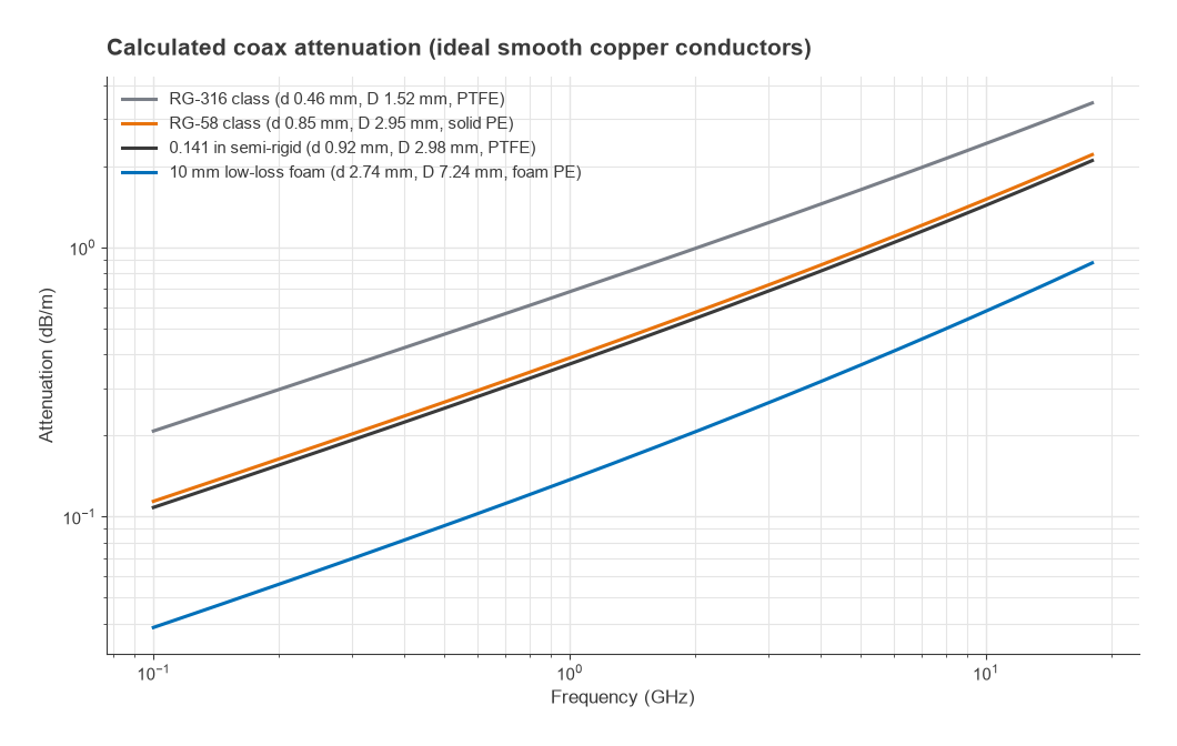
The ideal calculation agrees well with solid-outer cables such as semi-rigid and foil-plus-braid low-loss types. Braided and stranded cables, including most RG-58 and RG-316 constructions, measure noticeably higher because of braid coverage, stranding, plating and steel-cored centre conductors, so final link budgets should use the manufacturer’s attenuation curve. Other selection factors include phase stability with flexing and temperature for phased arrays and test cables, power rating, shielding effectiveness, minimum bend radius and outdoor UV and water resistance.
Choosing a connector
- Choose an interface rated comfortably above the highest frequency of interest, including harmonics that must be measured.
- Match the impedance of the system: 50 Ω for nearly all RF and microwave work, 75 Ω for video and cable TV.
- Choose Type N, TNC, 4.3-10 or 7/16 DIN for outdoor, high-power or low-PIM installations.
- Choose SMA for general modules to 18 GHz, and 2.92 mm or 2.4 mm when the design reaches 26.5 to 50 GHz. Millimetre-wave design issues are covered in mmWave radio architectures.
- Use snap-on micro-coaxial connectors only for internal links that are rarely disconnected.
Frequently asked questions
What are the types of RF connectors?
The common families are bayonet and snap-on types (BNC, SMB, MCX, MMCX and micro-coaxial), threaded general-purpose types (SMA, TNC, Type N), high-power low-PIM types (7/16 DIN, 4.3-10), 75 Ω video types (F, 75 Ω BNC), and precision air-line types (3.5 mm, 2.92 mm, 2.4 mm, 1.85 mm, 1.0 mm) for test above 18 GHz.
What frequency is SMA good for?
Standard SMA connectors are typically rated to 18 GHz, and well-made parts can be used to about 26.5 GHz. The limit comes from the TE11 mode in the PTFE-filled line, which begins near 25 GHz for SMA dimensions. Above that, 3.5 mm or 2.92 mm connectors are needed.
Can SMA mate with 2.92 mm connectors?
Yes, SMA, 3.5 mm and 2.92 mm connectors mate mechanically. The combination is limited to the lower-rated part’s frequency, and a worn or out-of-tolerance SMA can damage a precision connector, so pin depth should be checked before mating to test equipment.
Why is connector torque important?
Torque sets how firmly the outer conductors meet, which controls the electrical length and reflection of the joint. Consistent torque gives repeatable measurements, too little leaves a gap, and too much can permanently deform the contacts.
Related topics
Connectors usually sit between instruments and the parts being measured, as described in VNA basics and measuring radio performance. Other building blocks in the same section include RF attenuators and directional couplers, all collected in the RF passive components hub. Short definitions are in the wireless terms glossary.