

A constellation diagram is a plot of a digitally modulated signal’s samples in the complex I/Q plane, taken at the symbol decision instants, so each transmitted symbol appears as a point. Reading one means comparing the measured cloud of points with the ideal grid: the size, shape and position of each cluster reveal noise, phase noise, IQ imbalance, compression and other impairments in the radio.
An eye diagram shows the same signal along the time axis, overlaying many symbol periods of one channel so that timing errors and intersymbol interference become visible. The two views complement each other and are the first things most engineers look at when a link misbehaves. This page explains how both are built, how the error vector is defined, and the characteristic signature of each common impairment. It extends the digital modulation overview within the wider RF design map.
What the I/Q Plane Represents
Any bandpass signal can be written as s(t) = I(t) cos ωct − Q(t) sin ωct, or as the real part of the complex envelope I(t) + jQ(t) multiplied by ejωct. A digital modulator maps groups of bits to particular values of I + jQ. In PSK the points lie on a circle; in QAM they form a square or cross-shaped grid. The distance of a point from the origin is the symbol amplitude and its angle is the carrier phase.
A receiver recovers I and Q with an IQ demodulator or by digital downconversion, filters them with the matched filter, and samples once per symbol at the instant of maximum eye opening. Plotting those samples as points gives the constellation. Plotting the continuous I or Q waveform, folded every one or two symbol periods, gives the eye diagram.
Reading a Constellation Diagram
The ideal points are usually scaled so that the average symbol power is one. For square M-QAM the minimum spacing between neighbouring points is then
dmin = √(6 / (M − 1))
which gives 0.632 for 16-QAM and 0.218 for 64-QAM. The receiver decides which symbol was sent by finding the nearest ideal point, so the decision boundaries lie halfway between neighbours. A symbol error occurs when noise or distortion pushes a received point across a boundary, a distance of dmin/2. Higher-order constellations pack points more tightly for the same average power, which is why they need a higher SNR.
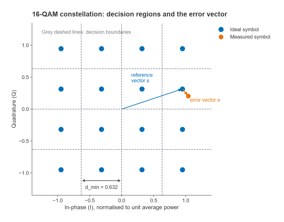
When reading a measured plot, check these in order:
- Cluster size: round, equal-sized clouds on every point indicate additive noise.
- Cluster shape: arcs centred on the origin indicate phase noise; arcs growing with amplitude point to a phase error that scales with radius.
- Grid geometry: a rectangle instead of a square or a skewed grid indicates IQ gain or phase imbalance.
- Outer points: corners pulled inward or rotated relative to inner points indicate compression and AM-PM.
- Origin: the whole grid shifted from the centre indicates carrier leakage or DC offset.
- Spinning: a constellation that rotates continuously indicates an uncorrected frequency offset.
Error Vector Magnitude
The error vector for symbol n is the difference between the measured point and the ideal point it was decided to be, en = rn − sn. Root-mean-square EVM normalises the average error power to the average reference power:
EVMrms = √( Σ|en|2 / Σ|sn|2 )
It is quoted in percent or in dB as 20 log(EVM). Before computing it, analysers normally remove the average gain, average phase, frequency offset and symbol timing error, so EVM reflects distortion rather than simple scaling. Some standards normalise to the peak symbol power rather than the average, which gives a smaller number for the same signal, so the definition has to be stated. The closely related modulation error ratio is MER = −20 log(EVMrms) dB when both use average power.
For additive white Gaussian noise alone, EVMrms ≈ 1/√SNR, with SNR measured at the decision point. An SNR of 30 dB gives 3.16 % and 20 dB gives 10 %. Independent impairments add in power, so the total EVM is the root-sum-square of the individual contributions. The link between EVM and waveform requirements is developed further in Radio Architectures Part 16.
Worked Example: An EVM Budget
A 64-QAM receiver has an SNR of 30 dB at the slicer, an LO with 1° rms integrated phase error, and an IQ demodulator with 0.5 dB gain imbalance and 3° phase imbalance.
- Noise: 1/√1000 = 3.16 %.
- Phase noise: σφ = 1° = 0.01745 rad, giving about 1.75 %.
- IQ imbalance: with gain ratio g = 100.5/20 and phase error φ = 3°, the image rejection ratio is IRR = (1 + 2g cos φ + g2) / (1 − 2g cos φ + g2) = 28.2 dB. The image term behaves like a correlated error at 10−28.2/20 = 3.9 %.
- Total: √(3.162 + 1.752 + 3.892) = 5.3 %, or MER ≈ 25.5 dB.
Without the IQ imbalance the figure would be 3.6 %. The example shows why receivers that rely on analog IQ paths usually include digital IQ correction, a point developed in image rejection and zero-IF receivers.
Impairment Signatures on a Constellation
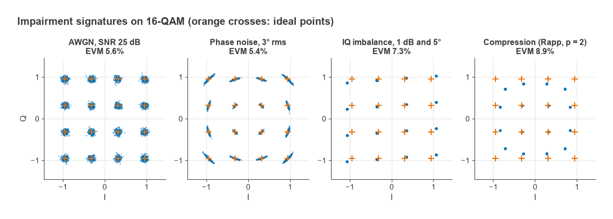
Figure 2 shows 16-QAM with four impairments applied one at a time in simulation. Each has a distinct shape, which is the main diagnostic value of the constellation view.
Additive Noise
Thermal noise, quantisation noise and wideband interference produce circular, Gaussian clouds of equal size on every point. At 25 dB SNR the simulated EVM is 5.6 %, matching 1/√SNR. If the clouds are circular but larger on some points than others, the noise is not additive and something else is involved.
Phase Noise
Phase noise on the LO rotates each received point by a random angle. The clusters stretch into arcs centred on the origin, and since the displacement is the angle times the radius, outer points smear more than inner points. For small angles EVM ≈ σφ in radians, so 3° rms gives about 5.2 %; the simulation, which includes a little additive noise, shows 5.4 %. Slow phase wander that the carrier recovery loop tracks does not appear, which is why only phase noise outside the tracking bandwidth matters for EVM.
IQ Imbalance
A gain mismatch between I and Q stretches the grid into a rectangle, and a phase error between the two LO paths skews it into a parallelogram. With 1 dB and 5° the IRR is 22.8 dB and the simulated EVM is 7.3 %. Unlike noise, the error is deterministic: the same symbol always lands in the same wrong place, so the clusters stay tight but displaced. Carrier leakage, the LO feeding through to the output, adds a constant offset that moves the whole grid away from the origin.
Compression and AM-PM
A compressing amplifier reduces the gain for high-amplitude symbols, so the corner and edge points move toward the origin while the inner points stay put. Because the analyser normalises to average gain, the inner points can appear slightly expanded. The simulated Rapp amplifier with p = 2 gives 8.9 % EVM. If the amplifier also has AM-PM conversion, the outer points also rotate relative to the inner ones. These errors grow quickly with drive and are the reason high-order QAM transmitters run with back-off from saturation.
Eye Diagrams
An eye diagram is built by triggering an oscilloscope, or slicing a captured waveform, at the symbol rate and overlaying successive traces of the I or Q channel, usually two symbol periods wide. For a binary or per-axis multilevel signal the traces form one or more open eyes. The vertical opening at the sampling instant is the noise margin, the horizontal opening is the timing margin, and the thickness of the crossing points shows jitter.
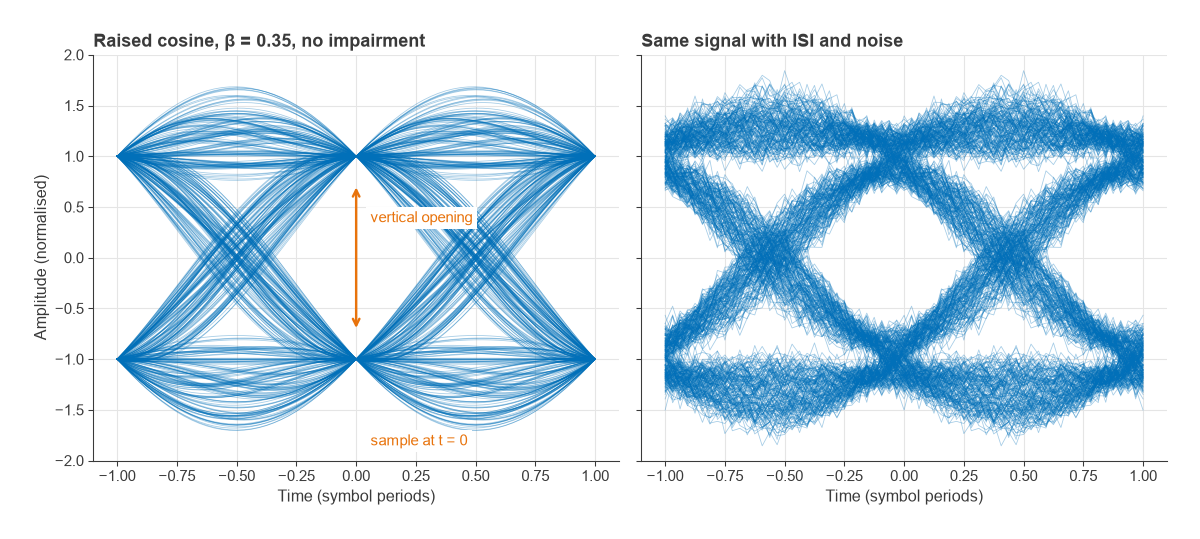
Pulse shaping determines how clean the eye can be. A raised-cosine overall response with roll-off β has zero intersymbol interference at the ideal sampling instants and occupies a bandwidth of (1 + β)Rs at RF. A 10 Msymbol/s signal with β = 0.35 therefore occupies 13.5 MHz. In practice the transmit and receive filters are each root raised cosine, so the eye at the transmitter output is not fully open; only after the matched filter does the full raised-cosine response appear. In the left half of Figure 3 every trace passes exactly through ±1 at t = 0.
The right half adds a one-pole low-pass filter, standing in for a channel or analog filter that is too narrow, plus noise. Each symbol now leaks into its neighbours, the traces no longer converge at t = 0, and the smallest sample magnitude in the simulation falls from 1.0 to about 0.57. That closure translates directly into a loss of noise margin. Eye diagrams are most useful for spotting timing problems, filter bandwidth errors and ISI. The constellation is better at separating amplitude and phase impairments, so the two are usually used together, as described in Radio Architectures Part 20.
Constellations for OFDM Signals
In an OFDM system the constellation is formed after the FFT, from the subcarrier symbols, not from the time-domain waveform. Every impairment is averaged over many subcarriers. Phase noise appears partly as a common rotation of all subcarriers, which pilots can correct, and partly as inter-carrier interference that looks like extra noise. A per-subcarrier EVM plot is the OFDM counterpart of the eye diagram: a rise at the band edges suggests filter ripple or group delay, and a spike near the centre suggests DC offset or LO leakage.
Frequently Asked Questions
How do you read a constellation diagram?
Compare the measured points with the ideal grid. Round clouds of equal size indicate noise, arcs indicate phase noise, a rectangular or skewed grid indicates IQ imbalance, and outer points pulled inward indicate compression. The overall spread is summarised by EVM.
What is the difference between a constellation diagram and an eye diagram?
A constellation plots I against Q at the sampling instants, so it shows amplitude and phase errors of each symbol. An eye diagram plots one channel against time over a few symbol periods, so it shows timing margin, jitter and intersymbol interference.
How is EVM related to SNR?
When additive noise is the only impairment, EVMrms ≈ 1/√SNR, so 30 dB SNR corresponds to about 3.2 % EVM. MER in dB equals the SNR at the decision point under the same conditions. Other impairments add to the error power and raise the EVM above that value.
Why does phase noise make arcs?
Phase noise rotates each symbol about the origin by a small random angle. Points at larger radius move further for the same angle, so the clusters become arcs that are longer at the corners of the constellation.
Related Topics
The modulation formats themselves are covered in QAM, PSK and phase modulation. For the hardware behind the impairments, see IQ modulators and demodulators, phase noise and AM-PM conversion. The wireless terms glossary defines EVM, MER and related abbreviations.