


Quadrature amplitude modulation (QAM) sends data by varying the amplitude of two carriers at the same frequency, 90 degrees apart, so that each symbol is a point on a two-dimensional grid. Its main advantage is spectral efficiency: M-QAM carries log2M bits per symbol, far more than binary schemes in the same bandwidth. The cost is a higher required SNR and tighter demands on linearity and phase noise.
QAM is one branch of the digital modulation techniques used in radio, and it is the constellation carried on the subcarriers of OFDM.
QAM Fundamentals: In-Phase and Quadrature Carriers
A QAM signal is the sum of a cosine and a sine, each scaled by a baseband level:
s(t) = I(t) cos(2πfct) − Q(t) sin(2πfct)
Cosine and sine are orthogonal over a symbol period, so a receiver that multiplies by each in turn and integrates recovers I and Q independently. Two data streams share one channel without interfering. In hardware this is an IQ modulator: two DACs, two mixers, and a local oscillator split into 0 and 90 degree paths.
Each symbol takes one of √M levels on each axis for square constellations. 16-QAM uses levels ±1 and ±3 on I and Q, which gives 16 points and four bits per symbol. Gray coding labels neighbouring points so that they differ by one bit, which means a symbol error to an adjacent point usually costs a single bit.
Normalising the 16-QAM constellation
Average power of the levels ±1, ±3 is (12 + 32)/2 = 5 per axis, or 10 for I and Q together. Dividing by √10 gives unit average power. The levels become ±0.316 and ±0.949, and the spacing between adjacent points is 2/√10 = 0.632. Corner points have power 18/10, which is 2.55 dB above the average.
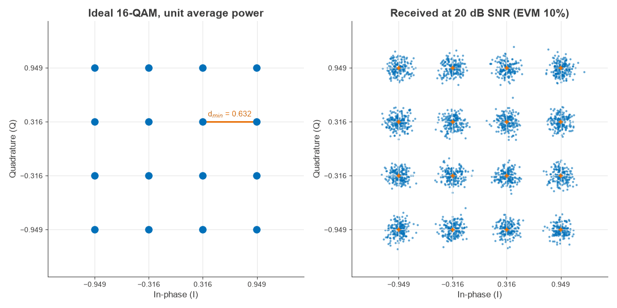
Constellation Size, Bit Rate and Minimum Distance
Each doubling of M adds a bit per symbol and shrinks the distance between points at fixed average power. The minimum distance dmin is what noise has to cross to cause an error, so it controls the required SNR.
| Constellation | Bits per symbol | dmin at unit power | Relative to QPSK (dB) | Peak/average (dB) |
|---|---|---|---|---|
| QPSK | 2 | 1.414 | 0 | 0 |
| 16-QAM | 4 | 0.632 | −6.99 | 2.55 |
| 64-QAM | 6 | 0.309 | −13.22 | 3.68 |
| 256-QAM | 8 | 0.153 | −19.29 | 4.23 |
| 1024-QAM | 10 | 0.077 | −25.33 | 4.50 |
Going from 64-QAM to 256-QAM adds two bits per symbol, a 33% rate increase, at the price of about 6 dB of distance.
The bit rate follows from the symbol rate. At 10 Msym/s, 64-QAM gives a gross rate of 60 Mbit/s. A rate 3/4 code leaves 45 Mbit/s of user data. Root-raised-cosine filtering at α = 0.25 occupies 10 × 1.25 = 12.5 MHz, for a net spectral efficiency of 3.6 bit/s/Hz.
Bit Error Rate of QAM in Noise
For Gray-coded square M-QAM in AWGN, with k = log2M, a close approximation is:
BER ≈ (4/k)(1 − 1/√M) Q(√(3k/(M−1) · Eb/N0))
For QPSK the expression reduces to the exact Q(√(2Eb/N0)). The conversion between the bit and symbol views is Es/N0 = Eb/N0 + 10log10k, described in more detail under SNR and Eb/N0.
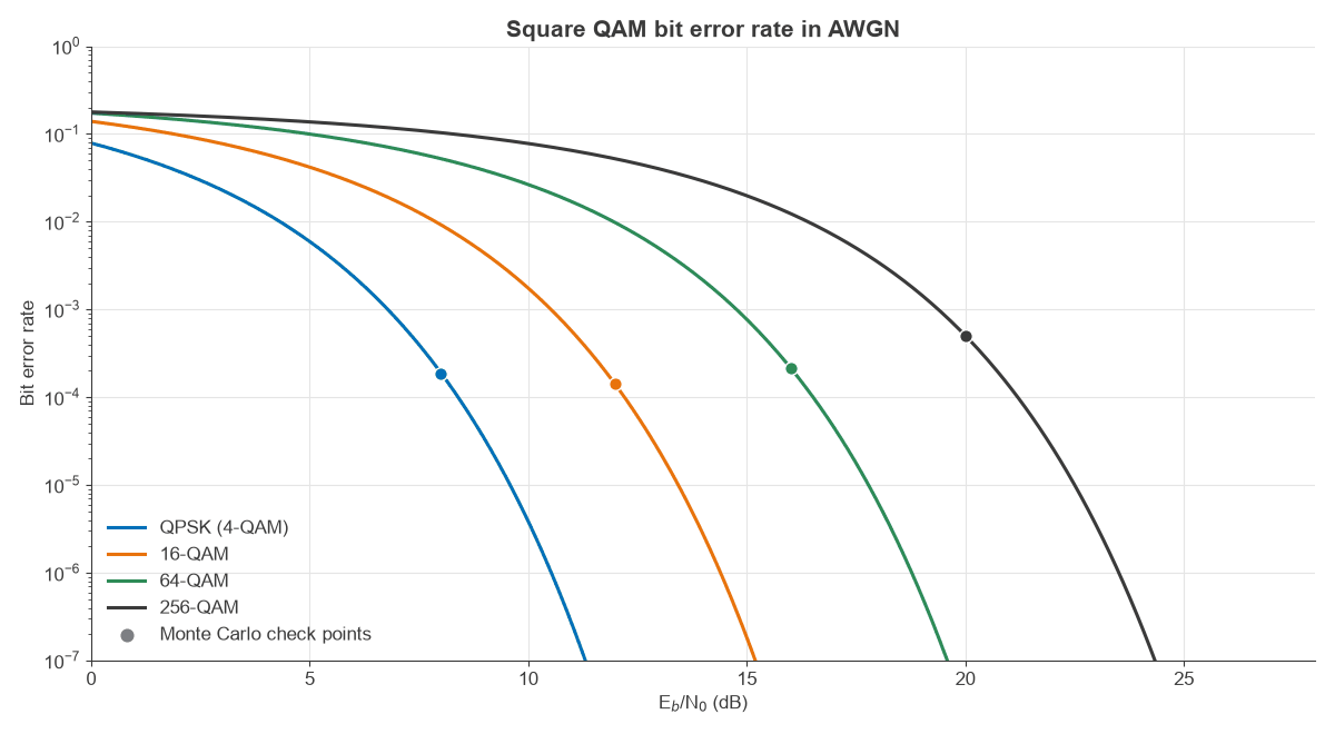
The dots in Figure 2 are Monte Carlo simulations of four million Gray-coded symbols, used to check the formula. They land on the curves:
| Case | Formula BER | Simulated BER | Formula EVM (%) | Simulated EVM (%) |
|---|---|---|---|---|
| QPSK, Eb/N0 = 8 dB | 1.91 × 10⁻⁴ | 1.84 × 10⁻⁴ | 28.15 | 28.15 |
| 16-QAM, 12 dB | 1.39 × 10⁻⁴ | 1.42 × 10⁻⁴ | 12.56 | 12.56 |
| 64-QAM, 16 dB | 2.17 × 10⁻⁴ | 2.16 × 10⁻⁴ | 6.47 | 6.47 |
| 256-QAM, 20 dB | 5.05 × 10⁻⁴ | 5.04 × 10⁻⁴ | 3.54 | 3.54 |
At a BER of 10−6 the required Eb/N0 is 14.40 dB for 16-QAM, 18.78 dB for 64-QAM and 23.51 dB for 256-QAM. Error correction in a real link reduces these by several dB.
EVM: The Practical Measure of QAM Quality
Error vector magnitude (EVM) compares each received symbol with its ideal point. RMS EVM, normalised to average constellation power, is:
EVM = √(mean|error vector|2 / mean|ideal point|2)
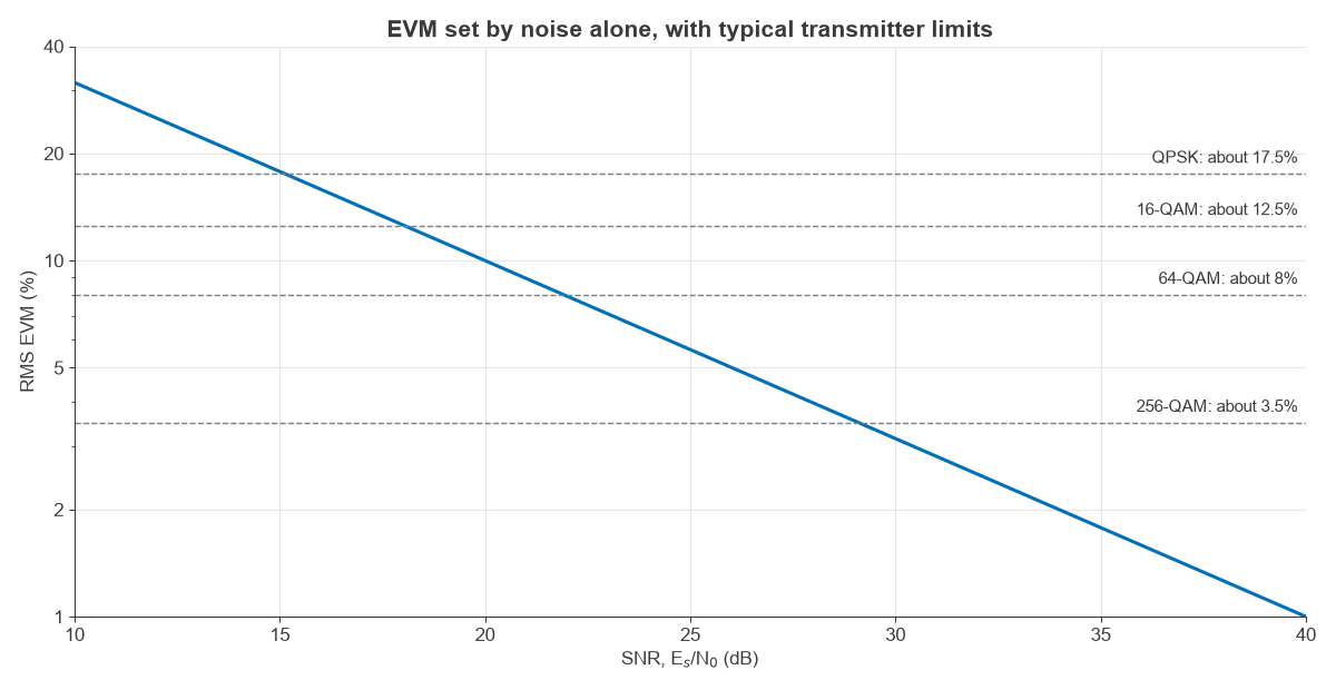
If the error is entirely noise, EVM = 10−SNR/20. So 20 dB gives 10%, 30 dB gives 3.16%, and 35 dB gives 1.78%. Figure 3 plots that line against typical transmitter limits. Cellular standards use limits of roughly 17.5% for QPSK, 12.5% for 16-QAM, 8% for 64-QAM and 3.5% for 256-QAM. Treat these as approximate and check the current specification for a given product class.
Worked example: from EVM to bit error rate
A 64-QAM signal arrives with 5% RMS EVM, and the error is close to Gaussian.
- Equivalent SNR: −20log10(0.05) = 26.02 dB.
- Eb/N0: 26.02 − 10log10(6) = 18.24 dB.
- Uncoded BER from the formula: 3.7 × 10⁻⁶.
At the 8% limit, the same steps give 21.94 dB, 14.16 dB and a BER of 1.9 × 10⁻³. The EVM limit therefore does not guarantee a clean uncoded link; it leaves the error correction code with work to do, plus margin for the channel. A real EVM floor from distortion is not exactly Gaussian, so these BER values are estimates.
Worked example: a transmitter EVM budget
Independent impairments add as powers, so percentages combine by root-sum-square. Consider a transmitter with these contributors:
- Phase noise of 1 degree RMS: 0.01745 rad, or 1.75%.
- Residual IQ imbalance and LO leakage: 1.5%.
- Power amplifier compression at the chosen back-off: 3.0%.
- Noise and spurs at 35 dB SNR: 1.78%.
The total is √(1.752 + 1.52 + 3.02 + 1.782) = 4.18%, or −27.6 dB. That leaves plenty of room against a 64-QAM limit of about 8%, but misses a limit of about 3.5% for 256-QAM. Backing off the amplifier is usually the first move, and PA linearization recovers some of the lost output. Modulation, EVM and PAPR covers this trade in depth, and Measuring Radio Performance covers how to measure it.
Advantages and Limits of QAM
QAM’s advantages are concrete. It packs more bits into a hertz than practical constant-envelope schemes, it fits the IQ architecture directly, and modulation order can change frame by frame, which is how adaptive links follow the channel.
The limits come from the same geometry. Closely spaced points respond to every impairment:
- Amplitude compression pulls corner points inward. AM-AM and AM-PM distortion also rotates them, and spectral regrowth raises ACLR.
- Phase noise smears the outer points along an arc, because a phase error moves a point by an amount proportional to its radius. See phase noise.
- IQ gain and phase imbalance skews the grid and creates an image.
QAM compared with PSK comes down to how the states are used. At four bits per symbol, 16-QAM needs about 4 dB less Eb/N0 than 16-PSK at a BER of 10−6, because points on a grid are further apart than points on a single ring. PSK still wins where a constant symbol amplitude matters and for low orders. Both are special cases of phase and amplitude modulation of a carrier.
Frequently asked questions
How many bits does 256-QAM carry?
256-QAM carries eight bits per symbol, since log2256 = 8. Compared with 64-QAM, that is a 33% increase in gross bit rate at the same symbol rate, for about 4.7 dB more Eb/N0 at a BER of 10−6.
What is a good EVM for QAM?
The answer depends on the order. Limits of about 8% for 64-QAM and 3.5% for 256-QAM are typical in cellular transmitters, and a good design leaves margin below those figures.
Is EVM normalised to average or peak power?
Normalisation differs between standards, and it changes the number. For 64-QAM, 5% referred to average power equals about 3.27% referred to the peak constellation point, since the peak sits 3.68 dB above the average. Always check which reference a data sheet uses.
Why does QAM need a linear power amplifier?
QAM carries information in amplitude as well as phase. A compressed amplifier moves outer points by more than inner points, which raises EVM and spreads energy into adjacent channels. Constant-envelope schemes such as FSK and GMSK avoid this but offer much lower spectral efficiency.
Related topics
The overview of digital modulation techniques compares QAM with its alternatives. Phase shift keying, phase modulation and OFDM are the closest neighbours. The RF noise and RF linearity sections cover the impairments that set the limits.