

A phased array steers its beam by applying a progressive phase shift or time delay across its elements, so that their signals add in phase in the chosen direction and cancel elsewhere, with no moving parts. Phased array design is the part of RF design that sets element spacing, beamformer type, phase resolution and physical construction so the array scans without grating lobes or excessive beam squint.
Electronically steered arrays used to belong mainly to radar. They now appear in 5G millimetre-wave handsets and base stations, satellite user terminals and automotive radar, which has made the hardware side of array design a routine RF engineering task. The theory of beamforming and its signal-processing side are covered in beamforming and in Radio Architectures Part 18: MIMO, Beamforming and Phased Arrays. This page concentrates on the decisions an RF designer makes when building the array itself. It sits under multiple antenna systems in the RF design reference.
How a phased array steers a beam
Consider a uniform linear array of N identical elements spaced d apart. A plane wave arriving from angle θ, measured from broadside, reaches each successive element with an extra path length of d·sinθ, which is a phase difference of kd·sinθ, where k = 2π/λ. If each element is given a phase shift that cancels this difference for a chosen angle θ0, all elements add coherently in that direction. The required progressive phase step is
Δφ = 2π (d/λ) sinθ0
The resulting array factor, which multiplies the pattern of a single element, is
AF(θ) = (1/N) |Σn=0N−1 exp[jn(kd·sinθ − Δφ)]|
For a uniformly weighted array, the half-power beamwidth at broadside is approximately 0.886λ/(Nd) radians, and it widens roughly as 1/cosθ0 when the beam is steered, because the projected aperture shrinks. The array gain over a single element is 10log(N) dB, and the first sidelobe of a uniform array sits about 13 dB below the main beam. Amplitude tapers such as Taylor or Chebyshev weightings lower the sidelobes at the cost of a slightly wider beam and a small loss of gain.
Worked example: a 16-element array at 28 GHz
At 28 GHz the free-space wavelength is c/f = 299.79/28 = 10.71 mm, so half-wavelength spacing is 5.35 mm and a 16-element row is about 86 mm long. To steer to 30°, the phase step is 360° × 0.5 × sin30° = 90° per element. To steer to 60°, it is 360° × 0.5 × sin60° = 155.9°.
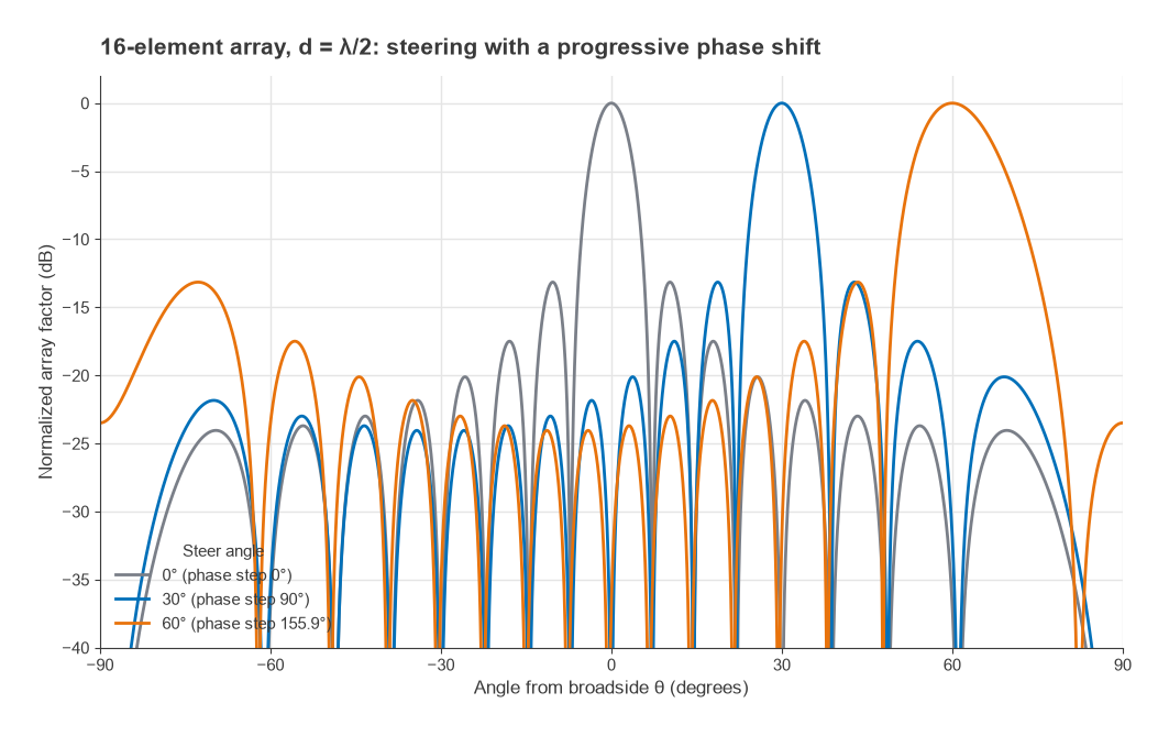
The approximate beamwidth formula gives 0.886 × 2/16 = 0.111 rad, or 6.35°, at broadside. Computing the array factor directly gives 6.35° at broadside, 7.35° at 30° and 13.0° at 60°, where the simple 1/cosθ0 scaling (12.7°) starts to underestimate. The array gain is 10log(16) = 12.0 dB, and the first sidelobe of this 16-element uniform array is at −13.1 dB. Figure 1 shows the three steered patterns.
Element spacing and grating lobes
The array factor is periodic in sinθ with period λ/d. When d is small, only one period falls within the visible region of −90° to +90°. When d is too large, a second full-height main beam, called a grating lobe, enters the visible region at
sinθg = sinθ0 − λ/d
To keep grating lobes out of real space for every scan angle up to θmax, the spacing must satisfy
d/λ < 1 / (1 + |sinθmax|)
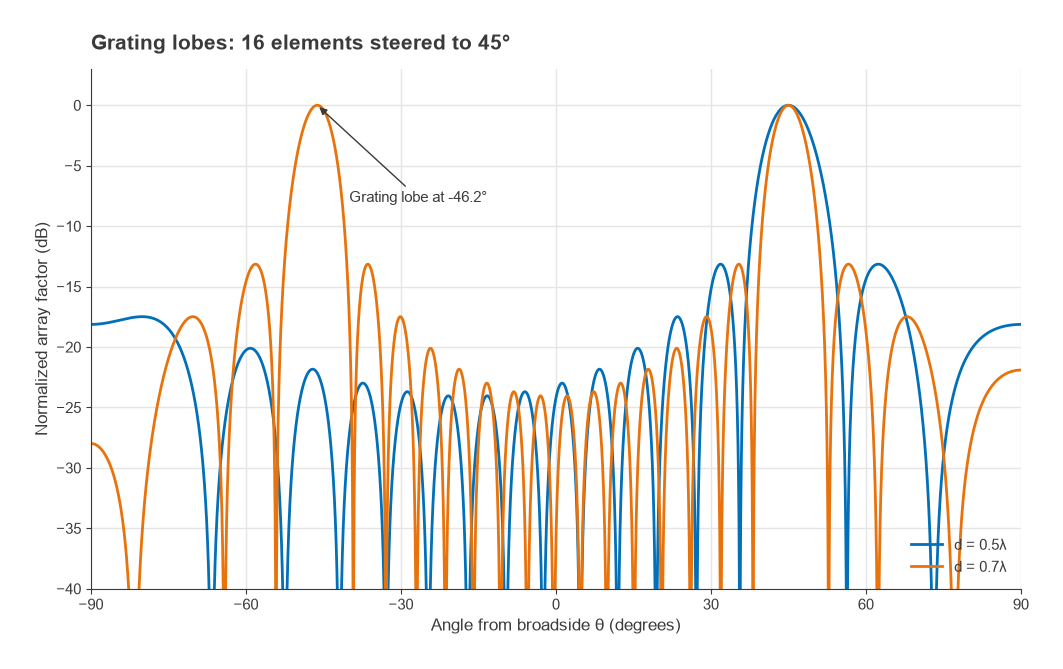
For a ±30° scan the limit is 0.667λ, for ±45° it is 0.586λ, and for ±60° it is 0.536λ. In practice designers keep some margin below the limit, because the grating lobe has a finite width and starts to raise the pattern before its peak reaches 90°. That is why λ/2 is the usual default for wide-scan arrays. With d = 0.7λ and a 45° steer, the grating lobe appears at sin−1(0.707 − 1.429) = −46.2°, as Figure 2 shows, while the same array at 0.5λ has no grating lobe at all.
Spacing below λ/2 avoids grating lobes but increases mutual coupling and reduces the area available to each element. Coupling makes the active impedance of each element change with scan angle, which can detune the matching and cause a scan blindness at particular angles. Element design therefore has to be checked in an array environment, usually with an infinite-array or finite-array EM simulation, rather than as a single isolated antenna. Single-element parameters are covered in antenna parameters, and the patch element common at millimetre-wave frequencies in patch antenna design.
Even without grating lobes, gain falls as the beam scans because the projected aperture shrinks. For an ideal element the loss is roughly 10log(cosθ0), about 3 dB at 60°; real element patterns usually fall faster, which is why many arrays limit scan to around ±45° to ±60°.
Phase shifters, time delay and beam squint
A phase shifter applies a fixed phase, which is equivalent to the correct time delay at only one frequency. At any other frequency the phase step no longer matches the path difference, and the beam points somewhere else:
sinθ(f) = (f0/f) sinθ0, and for small offsets Δθ ≈ (Δf/f0) tanθ0
This is beam squint. For the 16-element example steered to 30° at 28 GHz, the beam points at 31.2° at 27 GHz and 28.9° at 29 GHz, a shift of about ±1.2° against a 7.3° beamwidth. The edges of the band lose a fraction of a decibel of gain on target, which is usually acceptable. A larger array has a narrower beam, so the same squint becomes a bigger fraction of the beamwidth. As a rough guide, squint becomes a problem when the fractional bandwidth approaches the beamwidth in radians divided by tanθ0.
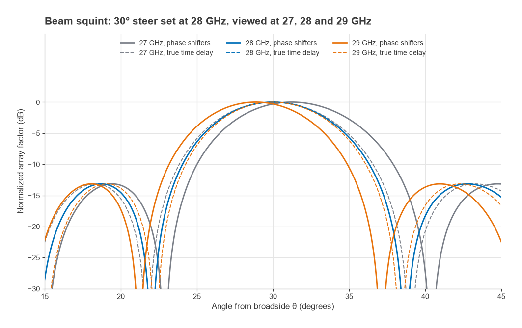
True time delay (TTD) removes squint by delaying each element by n·d·sinθ0/c, which is the correct compensation at every frequency. Figure 3 compares the two. TTD units are larger and lossier than phase shifters at RF, so large wideband arrays often use phase shifters at the element and TTD at the subarray level, or implement the delay digitally.
Phase shifter resolution
An n-bit digital phase shifter has a least significant bit of 360°/2n. If the quantization error is spread randomly across the elements, its RMS value is LSB/√12: 6.5° for 4 bits, 3.25° for 5 bits and 1.6° for 6 bits. The gain loss from random phase error is roughly exp(−σ2) with σ in radians, which is only about 0.014 dB for 5 bits. The larger effect is on sidelobes: when quantization errors repeat periodically across the array they form quantization lobes, and approximate rules place the peak of those lobes about 6 dB lower for each added bit. Low-sidelobe arrays therefore need more bits, or deliberate randomization of the rounding.
Beamforming architectures
Where the weighting happens determines cost, power and flexibility:
- Analog (RF) beamforming: phase shifters and variable-gain amplifiers at each element, combined at RF into one transceiver. Lowest power and cost per element, but one beam per RF chain.
- Digital beamforming: a full transceiver and data converter per element, with weights applied in DSP. Many simultaneous beams and TTD for free, at the highest power and data rate.
- Hybrid beamforming: analog subarrays, each feeding one digital chain. This is the common compromise in millimetre-wave base stations, and it links array design to the spatial multiplexing capability of the system.
In analog arrays the element-level front end is usually a beamformer IC containing, for several channels, a low-noise amplifier, power amplifier, T/R switch, phase shifter and gain control. Its noise figure and output power, multiplied across N elements, set the array’s G/T and EIRP. Transmit EIRP grows as 20log(N) for a fixed per-element power, because array gain and total power both scale with N. The surrounding millimetre-wave transceiver design is discussed in Radio Architectures Part 19: mmWave Radio Architectures.
Tile versus brick architectures
Physical construction is driven by the element pitch. In a brick architecture, circuit boards or modules run perpendicular to the aperture, each carrying the electronics for a column of elements. Depth is unconstrained, so components can be large and heat is easy to remove along the boards, but each board must fit within one element pitch in width. Bricks suit lower frequencies, where λ/2 is several centimetres, and high-power radar.
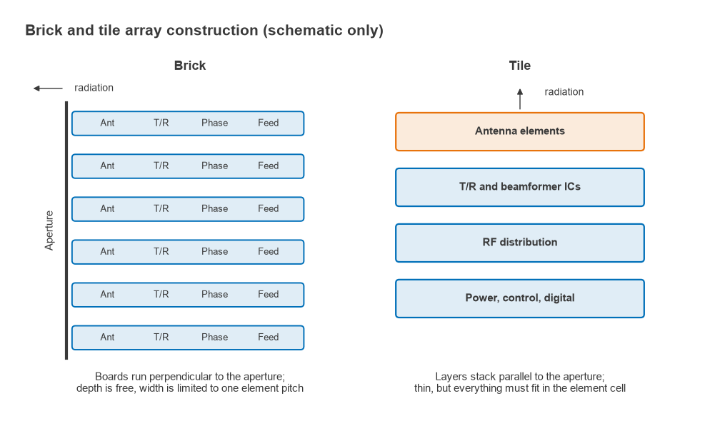
In a tile architecture, functional layers stack parallel to the aperture: antenna layer on top, beamformer ICs underneath, then RF distribution and power and control layers. Tiles are thin and suit planar, low-profile products, but every function must fit inside the element cell area. At 28 GHz that cell is about 5.35 mm square, so tiles are close to mandatory, and multi-channel beamformer ICs mounted directly under the antenna layer are the usual solution. Heat flows out through the back of a thin stack, so thermal design and the choice of PCB laminate become central. Figure 4 sketches both approaches.
Design steps
- Set the required beamwidth, gain or EIRP, and scan range from the link or radar budget.
- Choose element spacing from the grating lobe condition at the highest operating frequency and maximum scan angle.
- Size the array: N from gain and beamwidth, then per-element power and noise figure from EIRP and G/T.
- Check beam squint over the band and decide between phase shifters and time delay at each level.
- Choose phase and amplitude resolution from the sidelobe requirement, and select an amplitude taper.
- Design and simulate the element in an array environment, checking active match over scan.
- Pick tile or brick construction, then plan calibration, since channel-to-channel phase and gain errors must be measured and corrected.
Frequently asked questions
How does a phased array steer a beam?
Each element is driven with a phase that increases by a fixed step across the array, Δφ = 2π(d/λ)sinθ0. The signals then add in phase in the direction θ0 and partly cancel elsewhere. Changing the phase step moves the beam electronically, in microseconds or less.
Phase shifter vs true time delay: which should be used?
Phase shifters are smaller and cheaper but correct only at one frequency, so the beam squints across the band. True time delay is correct at all frequencies and is needed for wide instantaneous bandwidth or very large arrays. Many designs combine phase shifters at the element with time delay at the subarray.
Why is element spacing usually half a wavelength?
Grating lobes stay out of real space for all scan angles when d/λ is below 1/(1 + |sinθmax|). Half a wavelength meets that condition for scans approaching ±90°, which leaves comfortable margin at the ±45° to ±60° used by most practical arrays, while still leaving room for each element. Narrow-scan arrays can use wider spacing and fewer elements.
What is the difference between tile and brick arrays?
Brick arrays place electronics on boards perpendicular to the aperture, giving depth for components and cooling. Tile arrays stack layers parallel to the aperture, giving a thin assembly in which every function must fit inside one element cell. Millimetre-wave arrays are usually tiles because the cell is only a few millimetres across.
Related topics
Array design builds on multiple antenna systems and beamforming, and feeds directly into system work such as the 5G RF front end, radar and satellite RF design. Path loss and propagation at millimetre-wave frequencies are covered in Radio Architectures Part 17, and array terms are defined in the wireless terms glossary.