

Free-space path loss (FSPL) is the reduction in received power between two isotropic antennas separated by a line-of-sight path with no obstructions, reflections or absorption. It is the baseline propagation loss of every radio link: FSPL(dB) = 20log10(d) + 20log10(f) + 32.44, with d in kilometres and f in megahertz. Real links lose more, never less, than this figure on average.
The loss does not come from the medium. Free space absorbs nothing. It comes from geometry: power leaving a source spreads over an ever larger sphere, and a receiving antenna of finite size intercepts only a small part of it. This page derives the formula, explains why it grows with frequency, works a complete link example, and provides a calculator. It sits within the antennas and propagation section of the RF design reference.
The Free-Space Path Loss Formula
Derivation from spherical spreading
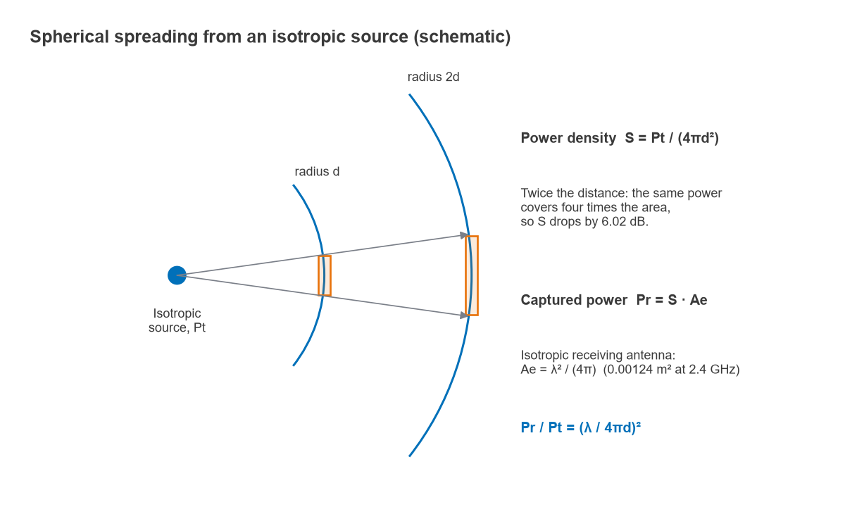
Start with a transmitter that radiates power Pt equally in all directions. At distance d that power is spread uniformly over a sphere of area 4πd2, so the power density is
S = Pt / (4πd2) (W/m2)
A receiving antenna behaves as if it collects all the power falling on a certain effective area Ae, so the received power is Pr = S · Ae. Antenna theory links effective area to gain through Ae = Gλ2/(4π). For an isotropic receiving antenna (G = 1) the effective area is λ2/(4π), and the ratio of received to transmitted power becomes
Pr / Pt = (λ / 4πd)2
Free-space path loss is the reciprocal of that ratio:
FSPL = (4πd / λ)2 = (4πdf / c)2
where c = 299,792,458 m/s. Adding real antenna gains Gt and Gr gives the Friis transmission equation, Pr = PtGtGr(λ/4πd)2, which in decibels is simply
Pr(dBm) = Pt(dBm) + Gt(dBi) + Gr(dBi) − FSPL(dB)
Practical forms of the equation
Taking 10log10 of (4πdf/c)2 separates distance, frequency and a constant that depends only on the units chosen:
FSPL(dB) = 20log10(d) + 20log10(f) + K, where K = 20log10(4π/c) adjusted for units
| Distance unit | Frequency unit | Constant K (dB) |
|---|---|---|
| km | MHz | +32.44 |
| km | GHz | +92.45 |
| m | MHz | −27.55 |
| m | Hz | −147.55 |
| statute miles | MHz | +36.58 |
The km/MHz constant computes to 32.448 dB, so some texts round it to 32.45 and others truncate to 32.44. The difference is 0.01 dB and has no practical effect. The most common error is mixing units, for example entering metres into the km/MHz form, which shifts the result by exactly 60 dB.
How Path Loss Scales with Distance and Frequency
Because distance and frequency each enter as 20log10, both obey the same two rules of thumb:
- Doubling the distance adds 20log10(2) = 6.02 dB of loss. Ten times the distance adds 20 dB.
- Doubling the frequency adds 6.02 dB, when the antennas keep the same gain. Moving from 2.4 GHz to 5.8 GHz adds 20log10(5800/2400) = 7.66 dB; moving to 28 GHz adds 21.34 dB.
The inverse-square law is the reason radio links reach so far compared with guided media. A coaxial cable loses a fixed number of dB per metre, so its loss grows linearly with length. Free space loses 6 dB per doubling, so going from 1 km to 2 km costs the same as going from 1 m to 2 m. A link that closes with 20 dB of margin can, in free space, be extended by a factor of 1020/20 = 10 in distance before the margin is gone.
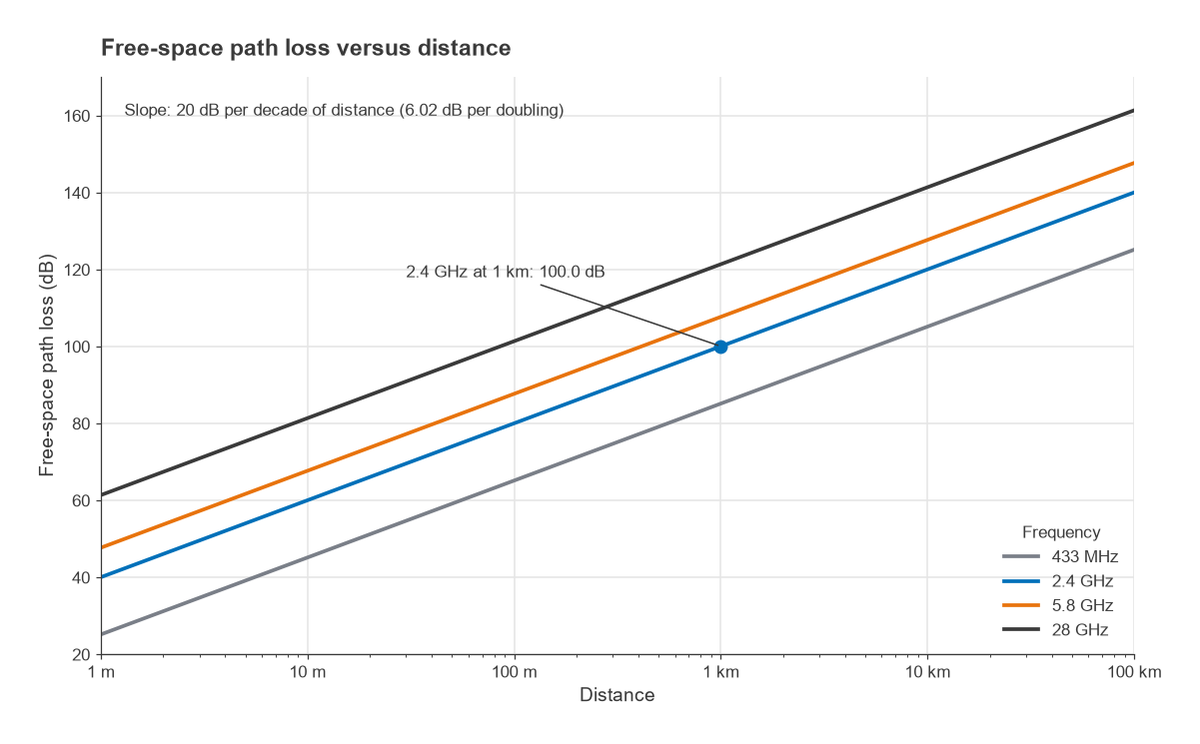
| Frequency | 100 m | 1 km | 10 km |
|---|---|---|---|
| 915 MHz | 71.7 dB | 91.7 dB | 111.7 dB |
| 2.4 GHz | 80.0 dB | 100.0 dB | 120.0 dB |
| 5.8 GHz | 87.7 dB | 107.7 dB | 127.7 dB |
Why Path Loss Increases with Frequency: the Aperture Explanation
The frequency term often causes confusion. Free space is not more lossy at higher frequencies, and the power density S = Pt/(4πd2) contains no frequency at all. The frequency dependence enters entirely through the receiving antenna.
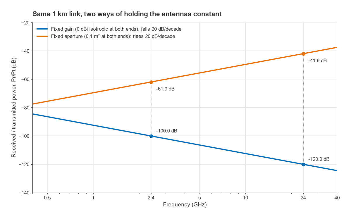
FSPL is defined between isotropic antennas, which have a fixed gain of 0 dBi at every frequency. The effective area of such an antenna is Ae = λ2/(4π). At 2.4 GHz, with λ = 0.1249 m, that is 0.00124 m2, roughly a 3.5 cm square. At 24 GHz the wavelength is ten times shorter and the effective area one hundred times smaller. A smaller collecting area intercepts less of the same power density, and that is the whole of the 20log10(f) term. A half-wave dipole, at about 2.15 dBi, shows the same behaviour: its effective area is 1.64λ2/(4π), and it shrinks with frequency because the dipole itself shrinks.
Hold the physical aperture constant instead and the conclusion reverses. A dish or flat panel of fixed area A has gain G = 4πA/λ2, which rises with f2. With fixed apertures At and Ar at both ends, the Friis equation becomes
Pr / Pt = AtAr / (λ2d2)
and the received power now improves by 20 dB per decade of frequency. For two 0.1 m2 apertures 1 km apart, Pr/Pt is −61.9 dB at 2.4 GHz and −41.9 dB at 24 GHz. The catch is that each 0.1 m2 aperture has a gain of about 19 dBi at 2.4 GHz and 39 dBi at 24 GHz, so its beam is very narrow and must be pointed accurately. This is why point-to-point microwave and millimetre-wave links use high-gain antennas, and why a mobile handset, whose antenna must cover all directions, sees the full frequency penalty.
Worked Example: a 2.4 GHz Link over 1 km
Consider a point-to-point link at 2.4 GHz with these parameters:
- Transmitter output Pt = +20 dBm (100 mW)
- Antenna gains Gt = Gr = 6 dBi, cable losses neglected
- Distance d = 1 km, clear line of sight
- Receiver sensitivity −90 dBm
Step 1, path loss: FSPL = 20log10(1) + 20log10(2400) + 32.44 = 0 + 67.60 + 32.44 = 100.04 dB.
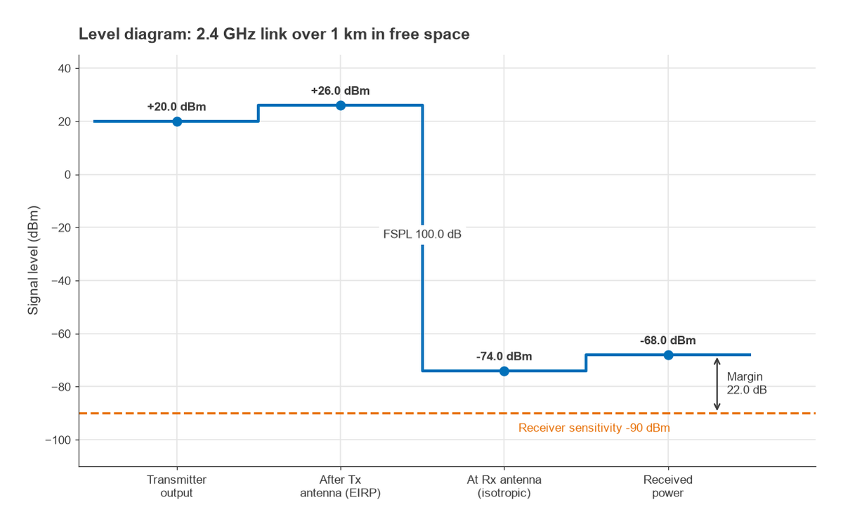
Step 2, received power: Pr = 20 + 6 + 6 − 100.04 = −68.04 dBm.
Step 3, margin: −68.04 − (−90) = 21.96 dB.
Step 4, maximum free-space range: the margin can absorb extra path loss of 21.96 dB, which corresponds to a distance factor of 1021.96/20 = 12.5. In ideal free space the link would close out to about 12.5 km. In practice that margin is kept to cover fading, rain, cable loss, antenna misalignment and Fresnel-zone obstruction, so the free-space range is an upper bound rather than a planning figure. A full treatment of those allowances belongs to the link budget, and the minimum usable signal comes from the receiver’s sensitivity.
Free-Space Path Loss Calculator
Enter the frequency and distance to get the path loss. Optionally add transmitter power and antenna gains to see the received power predicted by the Friis equation. The calculator uses the exact constant (32.448 dB for km and MHz).
Where the Free-Space Model Applies
The formula assumes three things, and each one breaks somewhere.
Far-field distance
Friis applies only in the far field of both antennas, where the wavefront is effectively plane and the field falls as 1/d. A common criterion is d > 2D2/λ, where D is the largest antenna dimension, together with d well beyond a few wavelengths. For a 0.6 m dish at 5.8 GHz (λ = 5.17 cm), 2D2/λ is about 13.9 m. Closer than that, the formula overestimates the coupling between the antennas, and near-field measurement or EM simulation is needed instead.
Clear first Fresnel zone
Line of sight between the antennas is not enough. Energy travels in an ellipsoidal region around the direct ray, the first Fresnel zone, and terrain, buildings or the ground intruding into it adds diffraction loss. A common planning guideline keeps at least 60 percent of the first Fresnel zone clear. Ground reflections can also add or cancel with the direct ray, and for long, low links the loss trends towards 40 dB per decade of distance rather than 20. These effects are covered in radio propagation basics.
No absorption or scattering
Atmospheric gases, rain, foliage and walls all absorb or scatter energy, and their effect grows with frequency. Below a few GHz, gaseous absorption is usually negligible over terrestrial distances. Above roughly 10 GHz, rain attenuation becomes a significant term, and near 60 GHz oxygen absorption is strong enough to dominate short links. These losses are added to FSPL in the link budget as separate line items.
Within those limits FSPL is exact, and it remains the reference against which empirical models for urban, indoor and terrain-dependent paths are expressed: most such models are written as free-space loss plus excess loss.
Frequently asked questions
What is free-space path loss?
It is the ratio of transmitted to received power between two isotropic antennas in an unobstructed, non-absorbing medium. It arises because radiated power spreads over a sphere of growing area while the receiving antenna collects power over a fixed effective area. In decibels it equals 20log10(d) + 20log10(f) + 32.44 for kilometres and megahertz.
Why does path loss increase with frequency?
Because the effective area of an antenna with a fixed gain is proportional to λ2. At higher frequencies a 0 dBi antenna is physically smaller and intercepts less of the same power density. If the physical aperture is held constant instead, gain rises with frequency and the received power actually increases.
How much does path loss increase when distance doubles?
By 6.02 dB in free space, since power density falls with the square of distance. Over real terrain with a strong ground reflection, the long-range trend can approach 12 dB per doubling, which is why free space gives the most optimistic range estimate.
Does free-space path loss include antenna gain?
No. FSPL is defined between isotropic antennas. Antenna gains are added separately in the Friis equation, Pr = Pt + Gt + Gr − FSPL, all in dB units. Gain definitions are covered on the antenna parameters page.
Related topics
Free-space loss is one line in a complete RF link budget, which can be explored with the link budget calculator. The antenna side of the equation continues in antenna gain, directivity and efficiency and patch antenna design. For the decibel arithmetic used throughout, see dB and dBm explained, and for the link between frequency and wavelength, frequency and wavelength.