


CSI-based power allocation in MIMO systems means dividing the transmit power among the channel’s spatial modes according to how strong each one is, instead of splitting it equally. With full channel knowledge at the transmitter the best rule is water-filling, which gives more power to strong modes and turns the weakest off. It helps most at low SNR, where it added about 85% to average capacity at -10 dB on a 4 × 4 Rayleigh channel, and almost nothing above 20 dB.
The MIMO and multiple antenna systems page gives the overview of MIMO itself, and MIMO capacity gives the general limit. This page deals with one design decision: how much power to send on each stream, given what the transmitter knows.
From a MIMO channel to parallel streams
Singular value decomposition splits a MIMO channel into independent paths:
H = UΣVH
If the transmitter precodes with V and the receiver combines with UH, the link becomes r separate channels, with r the rank of H. Stream i has power gain gi = σi2/N0, and given power pi it carries:
C = Σ log2(1 + pigi)
The sum of pi must not exceed the total power P. The question is how to choose each pi. Spatial multiplexing and MIMO precoding explain how the streams are formed. Here they are taken as given.
Equal power: what happens without CSI at the transmitter
A transmitter that knows nothing about H cannot favour any direction, so it splits power equally across antennas. The rate is then Σ log2(1 + (P/Nt)gi). This is the standard open-loop figure, and equal power is the optimal choice on an isotropic Rayleigh channel when the transmitter has no CSI.
Water-filling power allocation
With CSI at the transmitter, maximising C under the power limit gives the water-filling solution:
pi = max(0, μ – 1/gi)
The constant μ, the water level, is set so that the powers sum to P. For k active streams:
μ = (P + Σ 1/gi) / k
The name comes from a picture. Each stream is a vessel with a floor at height 1/gi. Pouring in total power P fills every vessel to the same level. A strong stream has a low floor and takes more power. A stream whose floor is above the water level gets none.
To compute it, sort the gains from highest to lowest and try all r streams. If μ falls below the highest floor in the set, drop the weakest stream and try again.
Worked example: four streams at P = 10
Take gains g = 6.0, 2.5, 1.0 and 0.25, so the floors are 0.167, 0.4, 1.0 and 4.0.
Trying all four gives μ = (10 + 5.567)/4 = 3.89, which is below the fourth floor of 4.0. So that stream is off. With three streams:
μ = (10 + 1.567)/3 = 3.856
Then p1 = 3.69, p2 = 3.46 and p3 = 2.86, which sum to 10. The rates are:
| Stream | Gain g | Water-filling power | Rate (b/s/Hz) | Equal power 2.5, rate (b/s/Hz) |
|---|---|---|---|---|
| 1 | 6.0 | 3.69 | 4.53 | 4.00 |
| 2 | 2.5 | 3.46 | 3.27 | 2.86 |
| 3 | 1.0 | 2.86 | 1.95 | 1.81 |
| 4 | 0.25 | 0 | 0 | 0.70 |
| Total | 10.0 | 9.75 | 9.37 |
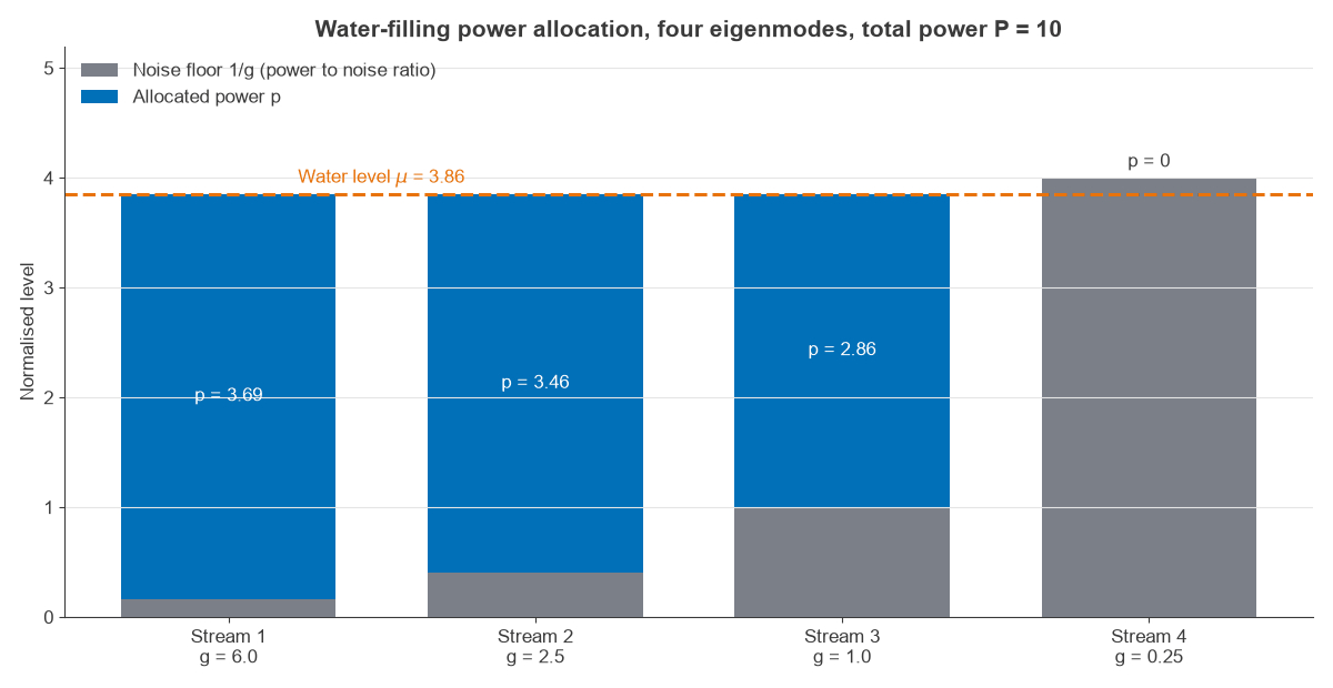
Water-filling gains 4.1% here. Now cut the total power by a factor of ten, to P = 1. Only streams 1 and 2 stay active, with μ = 0.783, p1 = 0.617 and p2 = 0.383. Capacity is 3.20 b/s/Hz against 2.43 b/s/Hz for equal power, a gain of 31.7%. It also beats putting all the power on stream 1, which gives 2.81 b/s/Hz. At P = 100 all four are active, and the two methods give 20.80 and 20.79 b/s/Hz, which is effectively no gain.
How much CSI-based power allocation is worth
That pattern holds on average. This table comes from 400,000 random 4 × 4 Rayleigh channels:
| Average SNR | Water-filling (b/s/Hz) | Equal power (b/s/Hz) | Gain | Active streams |
|---|---|---|---|---|
| -10 dB | 0.98 | 0.53 | 85% | 1.4 |
| 0 dB | 4.21 | 3.35 | 26% | 2.5 |
| 10 dB | 11.52 | 10.94 | 5% | 3.3 |
| 20 dB | 22.27 | 22.14 | 0.6% | 3.9 |
| 30 dB | 34.91 | 34.89 | under 0.1% | 4.0 |
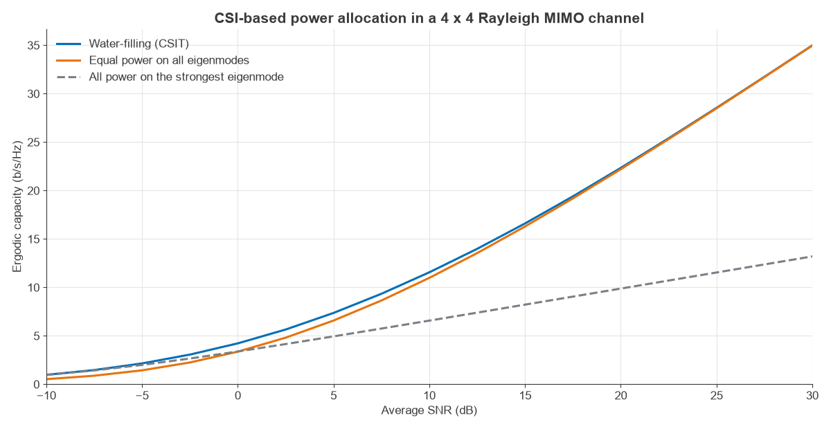
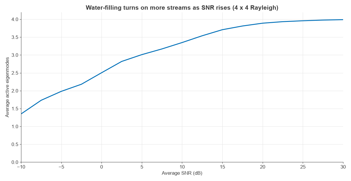
The two limits make sense. At low SNR, the water only covers the lowest floor, so water-filling becomes single-stream beamforming. At high SNR, the water is so deep that floor differences hardly matter, and all streams get about the same power. Most of the value is therefore in the middle and low range, which is also where cell-edge users sit.
Practical power allocation
Real systems depart from the textbook form in several ways.
- Discrete modulation. Modems use a finite set of modulation and coding schemes, not continuous rates. Gains are divided by an SNR gap Γ to reflect this. For the worked example with Γ = 3 dB, the rate falls from 9.75 to 7.31 b/s/Hz, and the power split shifts slightly.
- Rank adaptation does most of the work. Choosing how many streams to send captures most of the gain. Cellular links usually report a rank and a precoder, and split power equally across chosen layers, with link adaptation fitting a rate to each one.
- Per-antenna limits. Each power amplifier has its own peak limit, so the total-power form can ask for more than one PA can give. See RF amplifiers for the output limits.
- PAPR and EVM. High-order streams on the strongest mode need linearity, so a PA backed off for them gives up power elsewhere.
- Frequency domain. OFDM can water-fill across subcarriers as well. The formula is identical, with one vessel per subcarrier per stream. DSL does this in practice through bit loading.
- Multiuser allocation. Power now trades one user against another, and allocation is tied up with user selection. See user scheduling in MIMO systems.
Where power allocation sits in a real link
Power allocation is one of three decisions made together, along with rank and rate. For a given H, the link first picks how many streams to send, then how to divide the power, then which modulation and coding each stream can carry. The rate step sets what the result is worth, because an unused fraction of a modulation step is wasted. An engineer tuning a link therefore rarely adjusts powers alone. The useful quantity to check is the rate after all three decisions, measured against the capacity limit above.
Imperfect CSI
Water-filling trusts the gains it is given. If the CSI is wrong or old, power can go to a stream that has faded. Channel estimation errors shows how much that costs, and in a fast channel the transmitter may do better with statistical CSI: long-term average channel strengths and correlation, which change slowly and are cheap to feed back. Power then follows the average eigenmodes, not the instantaneous ones.
Frequently asked questions
What is water-filling in MIMO?
It is the capacity-achieving power allocation when the transmitter knows the channel. Power goes to the spatial streams so that power plus inverse gain is equal on every active stream, and streams below a threshold get none.
When does water-filling help most?
At low SNR and on channels with very unequal stream gains. In the 4 × 4 Rayleigh results above it added 85% at -10 dB and 26% at 0 dB, but under 1% at 20 dB.
Do 5G systems use water-filling?
Not in the pure form. They use rank adaptation, precoding and link adaptation, usually with equal power across layers, plus water-filling-like behaviour through scheduling and rank choice. These capture much of the gain with less signalling.
Does power allocation need channel state information?
Instantaneous allocation needs CSI at the transmitter. Without it, equal power is the sensible default. With only long-term CSI, power can follow the average channel. Channel state information covers how each kind is obtained.
Related topics
Massive MIMO spectral efficiency shows how power and user count interact at scale, and deep learning CSI feedback covers how CSI reaches the transmitter. The wider topic area is on the MIMO and RF design hubs.