


Spatial multiplexing is a MIMO technique that sends separate data streams from different antennas in the same time and frequency, using the spatial differences between propagation paths to tell them apart at the receiver. Its role in a MIMO system is to turn extra antennas into extra data rate, at up to min(Nt, Nr) times the single-stream slope. It competes for those same antennas with beamforming and spatial diversity, and the real limit on stream count is usually the channel, the hardware or the pilot budget.
This page is about that role: what spatial multiplexing is good for, what it gives up, and where the extra streams stop paying. The channel mathematics, SVD and receiver types are worked through in the companion article on spatial multiplexing, SVD and channel rank.
What is spatial multiplexing?
A radio with one antenna pair has one spatial channel. With several antennas at each end, and with paths that reach each receive antenna differently, the channel behaves like a set of parallel links in one bandwidth. Spatial multiplexing assigns a separate coded stream to each of those links. Nothing about the radio’s bandwidth or power budget changes, since total transmit power is shared between the streams.
Spatial multiplexing in MIMO depends on the receiver being able to separate those streams, which it does by estimating each transmit-to-receive path from pilots. If all paths looked the same, the streams would collapse into a single observation and could not be recovered. That is why scattering or carefully designed antenna geometry is required.
Spatial streams vs MIMO
The two terms are often confused. MIMO describes the antennas: a 4×4 radio has four transmit and four receive antennas. A spatial stream is an independent data sequence. A 4×4 link can carry one, two, three or four streams, and it changes that number with channel conditions. MIMO hardware sets the maximum, and the channel decides how many streams are useful at a given moment.
Spatial multiplexing gain
Spatial multiplexing gain is the slope of rate against SNR, measured in b/s/Hz per 3 dB. A SISO link at high SNR gains 1 b/s/Hz for each 3 dB, and a link with r usable streams gains r b/s/Hz. The maximum is:
rmax = min(Nt, Nr)
This is a multiplier on the slope of the curve, not a fixed rate multiplier. At low SNR, where capacity is close to linear in power, splitting power across streams brings little and can lose against sending one strong beam. The next section shows where that happens. MIMO capacity gives the formal treatment.
Spatial multiplexing and beamforming compared with diversity
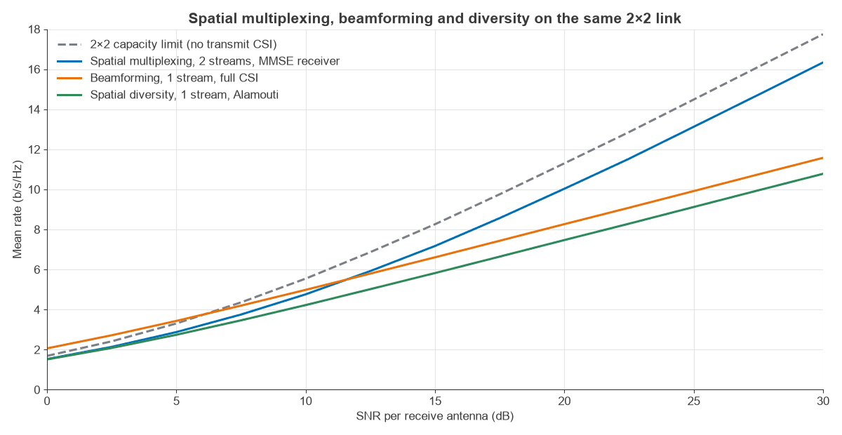
The same antennas can be used in three ways. Spatial multiplexing maximises rate, beamforming maximises SNR on one stream, and spatial diversity maximises reliability on one stream. Figure 1 compares them on a 2×2 Rayleigh link, using rates calculated over 200,000 channel draws at each table point.
| SNR | Multiplexing, 2 streams, MMSE | Beamforming, 1 stream, CSI | Diversity, Alamouti | Capacity, no CSI |
|---|---|---|---|---|
| 0 dB | 1.53 | 2.06 | 1.51 | 1.69 |
| 10 dB | 4.77 | 4.99 | 4.23 | 5.55 |
| 20 dB | 10.02 | 8.26 | 7.47 | 11.29 |
| 30 dB | 16.33 | 11.58 | 10.78 | 17.75 |
Values are in b/s/Hz. Below about 12 dB, one beamformed stream carries more than two multiplexed streams, assuming the transmitter has CSI. At 30 dB, multiplexing gives 41% more than beamforming. The diversity line needs no transmit CSI and sits about 0.8 b/s/Hz below beamforming at high SNR, because the transmit power is split without array gain.
Spatial diversity vs spatial multiplexing
Mean rate is only half of the comparison, since a fixed-rate service cares about outage. The table shows the fraction of channel states in which each mode falls below a target rate.
| Case | Multiplexing | Beamforming | Diversity |
|---|---|---|---|
| 3 b/s/Hz at 10 dB | 14.2% | 1.0% | 5.4% |
| 8 b/s/Hz at 20 dB | 21.6% | 34.3% | 75.0% |
At a modest target, multiplexing fades too often, because the weaker stream drags down the sum when the channel is poorly conditioned. At a high target, one stream is simply not enough, and multiplexing has the lowest outage. A good link adapts between these modes. The formal version of the trade-off is the diversity-multiplexing tradeoff: a rate that rises faster with SNR gives a shallower error slope. Diversity techniques covers the reliability side of this.
Limitations of spatial multiplexing
Streams do not keep adding rate forever. The practical limits fall into four groups: channel rank and conditioning, transceiver quality, pilot overhead and receiver processing.
Channel rank and antenna correlation
If antennas are correlated, or scattering is limited, some spatial links have too little gain to carry data. Line-of-sight paths at long range are the extreme case, with effectively one link regardless of antenna count. The spatial multiplexing article shows how a poorly conditioned channel loses rate at equal total gain, and MIMO capacity plots the loss against correlation.
EVM and hardware limits on each stream
Transmitter imperfections add noise that scales with the signal, so raising power does not raise that stream’s SINR beyond a ceiling. Error vector magnitude (EVM) sets the limit. With EVM as a power ratio E and a stream SNR of γ:
SINR = γ / (1 + E γ), which approaches 1/E at high SNR
The rate on one stream cannot exceed log2(1 + 1/E). That is 6.66 b/s/Hz at −20 dB EVM, 8.31 b/s/Hz at −25 dB and 9.97 b/s/Hz at −30 dB. Figure 2 applies this to a 4×4 Rayleigh channel, using equal power on the strongest eigenmodes and assuming full CSI.
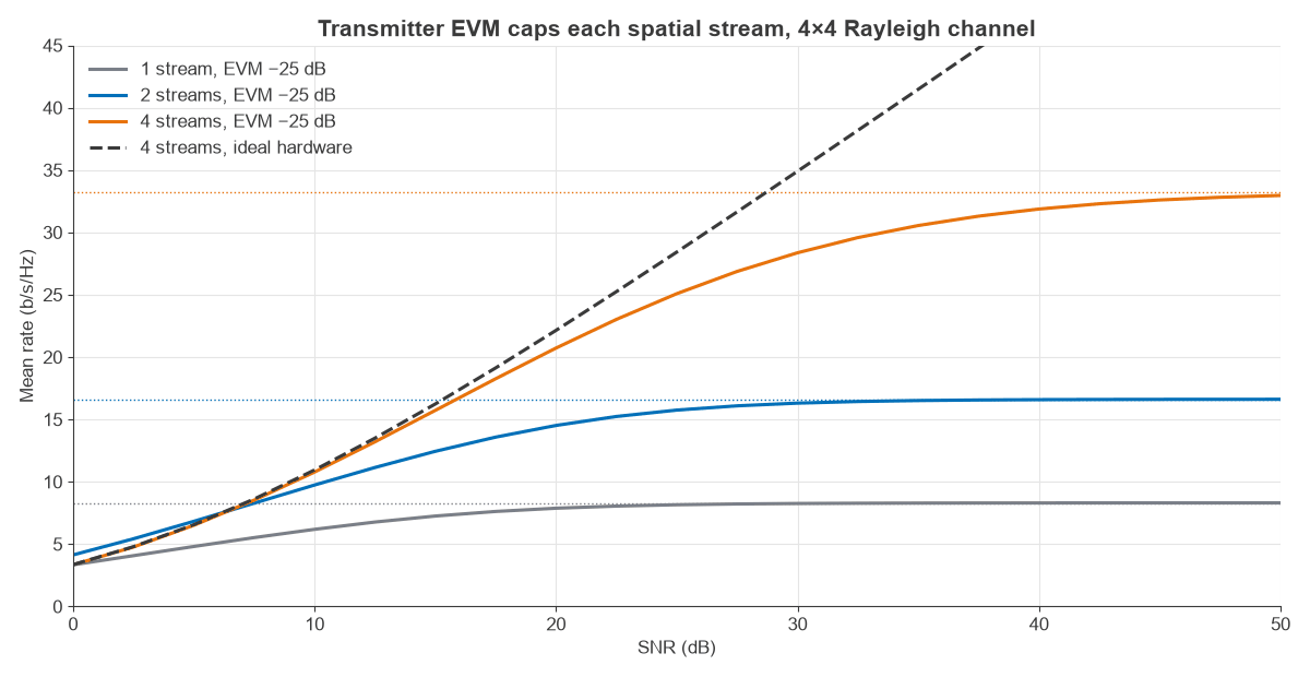
Worked example: at 30 dB SNR, four ideal streams give 34.9 b/s/Hz. With −25 dB EVM the same link gives 28.4 b/s/Hz, a loss of 19%. At 40 dB the ideal figure is 48.1 and the real one 31.9, a loss of 34%, with the extra 10 dB adding only 3.5 b/s/Hz. Improving EVM to −30 dB raises the 30 dB case to 31.6 b/s/Hz. High stream counts at high SNR are therefore often limited by the EVM budget, which sets the requirement for phase noise and PA linearity.
More streams also help reach the ceiling later. At 30 dB, one stream gives 8.26 b/s/Hz, which is within 0.6% of its −25 dB ceiling, while four give 28.37, which is 15% below theirs. Spreading power across streams keeps each one further from its ceiling.
Pilot overhead
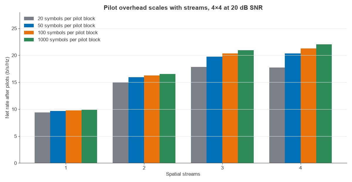
Each stream needs its own reference signal so that the receiver can estimate its path. If the channel stays constant for T symbols and k streams use one pilot symbol each, the useful fraction is 1 − k/T:
Rnet = (1 − k/T) Rk
| Streams | Rate, ideal | T = 20 | T = 50 | T = 100 | T = 1000 |
|---|---|---|---|---|---|
| 1 | 9.88 | 9.39 | 9.68 | 9.78 | 9.87 |
| 2 | 16.59 | 14.93 | 15.92 | 16.26 | 16.56 |
| 3 | 20.99 | 17.84 | 19.72 | 20.35 | 20.93 |
| 4 | 22.14 | 17.71 | 20.36 | 21.25 | 22.05 |
The fourth stream adds only 1.15 b/s/Hz before overhead, since it uses the weakest eigenmode. At T = 20, which is a fast-moving case with little channel coherence, it has a net cost: three streams beat four. For scale, a user moving at 30 km/h at 3.5 GHz has a Doppler shift near 97 Hz and a coherence time of about 4 ms, so the coherence length in symbols depends strongly on carrier frequency and speed. Real systems use pilot patterns far more efficient than one symbol per stream, but the scaling is the same.
Receiver limits
Separating streams takes signal processing, and linear detectors lose rate on poorly conditioned channels. Near-optimal MIMO detection algorithms cost more as stream count rises. Each stream also needs its own digital path, so a four-stream radio has four complete transceiver chains to power and calibrate.
Rank adaptation in practice
Radios measure the channel and report a preferred rank, modulation and precoder, then revise them as conditions change. In one design pass, the planner should ask four questions for each added stream:
- Does the channel have an eigenmode strong enough to carry it?
- Is the stream SNR well below the EVM ceiling, or is it already saturated?
- Does the extra rate exceed the added pilot and feedback overhead?
- Does the receiver have the processing budget to separate it?
If any answer is no, the antennas are better spent on array gain or diversity. A handset might run two streams at the cell edge and four near the base station on the same hardware. Beamforming and multiplexing are also combined, with several beams per user, in many base stations, and multiple antenna systems sets out how the three gains are divided.
Frequently asked questions
What is spatial multiplexing in simple terms?
It is sending different data on different antennas at the same time on the same frequency. The receiver uses the fact that each transmit antenna reaches it through a different path pattern to separate the signals. It increases data rate without using more spectrum.
What is the difference between spatial multiplexing and beamforming?
Spatial multiplexing sends several independent streams to raise rate. Beamforming sends one stream through all antennas with chosen phases to raise SNR. Beamforming wins at low SNR and multiplexing at high SNR, and the two can be combined.
Does spatial multiplexing need more power or bandwidth?
No. It shares the existing power across streams and uses the existing bandwidth. It needs extra antennas and transceiver chains at both ends, a channel with enough scattering, and enough SNR to split power without losing rate.
When should a radio not use spatial multiplexing?
Use fewer streams at low SNR, on correlated or line-of-sight channels, on fast-fading channels where pilots use too much of the coherence time, or where hardware EVM has already capped the rate. Rank adaptation makes this decision automatically in most systems.
Related topics
For the mathematics, read spatial multiplexing: SVD, channel rank and receivers. Adjacent articles cover MIMO capacity, beamforming, MIMO precoding and MIMO interference management. Hardware background is in MIMO, beamforming and phased-array architectures, and the antennas themselves are covered under antennas.