Understanding MIMO: Spatial Diversity and Spatial Multiplexing in Wireless Communication

Spatial diversity and spatial multiplexing are the two ways MIMO can spend its extra antennas. Spatial diversity sends the same information over several paths so that a link survives fades, while spatial multiplexing sends different data streams over those paths to raise the rate. A real radio has to choose between them, or blend them, on every frame.

This article is about that choice in MIMO wireless communication: what each mode gives, where one overtakes the other, and how a link switches between them. The signal theory behind streams is in spatial multiplexing in MIMO, and a general introduction is in MIMO and multiple antenna systems.

What is spatial multiplexing?

Spatial multiplexing transmits independent data streams from different antennas in the same band at the same time. In a channel with rich scattering, each receive antenna sees a different mix of the streams, and the receiver solves for them much like simultaneous equations. A link with N_t transmit and N_r receive antennas can carry at most min(N_t, N_r) streams, so a 2×2 link carries two. Doubling the streams doubles the slope of rate against SNR in decibels: at high SNR, 3 dB more power adds 2 b/s/Hz instead of 1.

What is spatial diversity?

Spatial diversity in MIMO sends coded copies of one stream through all the antenna paths. The 2×2 channel has four paths, so the Alamouti space-time code combined with two receive antennas gives diversity order 4. Rate is that of one stream, but outage falls as SNR^-4, so deep fades nearly vanish. The equivalent channel for Alamouti has power gain ‖H‖_F²/2, the sum of all four path powers shared between two transmitters, which gives:

R_div = log₂(1 + (ρ/2)‖H‖_F²)

A two-stream MMSE receiver gives a sum of per-stream rates:

R_mux = Σ_k -log₂[(I + (ρ/2)H^HH)^-1]_kk

Here ρ is total transmit power over noise per receive antenna. These two expressions are the basis of the comparison below.

Spatial diversity and spatial multiplexing compared

Property	Spatial diversity	Spatial multiplexing
Goal	Reliability	Peak rate
Streams on 2×2	1	2
Diversity order on 2×2	4 (Alamouti)	2 at best, with uncoded streams and an ML receiver
High-SNR rate slope	1 stream	2 streams
Needs rich scattering	For full diversity, uncorrelated paths	Yes, or rank falls to 1
Receiver	Simple linear combining	MMSE, successive cancellation or ML
Best conditions	Cell edge, fast movement	High SNR near the transmitter

Worked comparison: rate on a 2×2 link

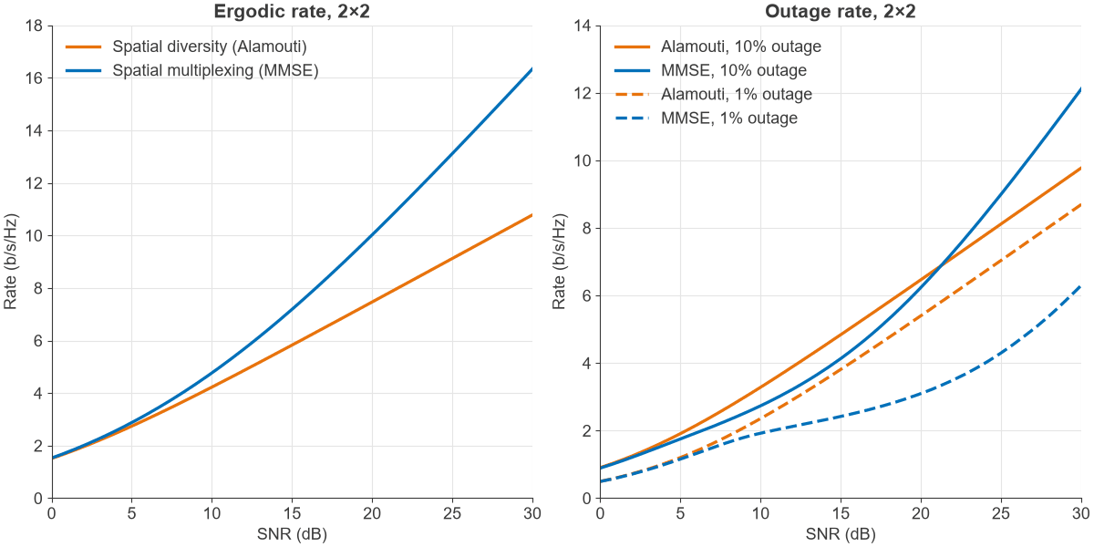
The table uses 1 million i.i.d. Rayleigh channel draws with open-loop transmission and power shared equally. “Outage rate” is the rate the channel supports in all but 1% or 10% of draws.

SNR	Alamouti ergodic	MMSE two-stream ergodic	Alamouti 10% outage	MMSE 10% outage	Alamouti 1% outage	MMSE 1% outage
0 dB	1.51	1.53	0.91	0.89	0.50	0.49
10 dB	4.23	4.77	3.28	2.73	2.36	1.92
20 dB	7.47	10.02	6.46	6.23	5.40	3.10
30 dB	10.78	16.33	9.77	12.10	8.69	6.30

All rates are in b/s/Hz. Three results follow.

• On average, multiplexing wins almost everywhere. The two curves are equal near 0 dB, and at 20 dB the two streams give 10.0 b/s/Hz against 7.5.
• When outage matters, diversity holds on far longer. The crossover for an MMSE receiver is about 21.3 dB at 10% outage. At 1% outage, it is close to 40 dB.
• The gap comes from the receiver as well as the channel. The capacity of the channel with no CSI, 11.3 b/s/Hz ergodic at 20 dB, beats the MMSE receiver at 10.0. A stronger receiver moves the crossover to lower SNR.

Worked in 20 MHz at 20 dB SNR, the choice is 149 Mb/s for Alamouti against 200 Mb/s for two streams on average, but at 1% outage it is 108 Mb/s against 62 Mb/s. Neither mode dominates, so the design goal decides.

Comparison at the same rate

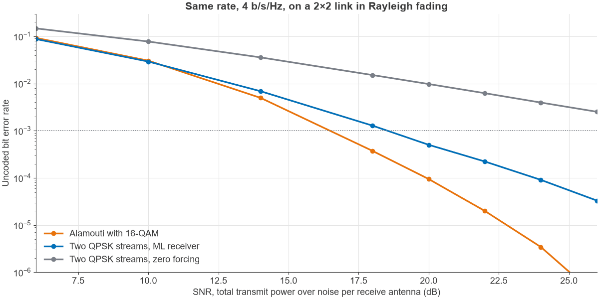
A second way to compare is to fix the rate and look at errors. For 4 b/s/Hz on a 2×2 link, Alamouti needs 16-QAM, since it sends one symbol per use, and multiplexing needs QPSK on two streams. Figure 2 shows uncoded simulation results from 800,000 channel draws per point.

Scheme at 4 b/s/Hz	SNR for BER 10-3
Alamouti, 16-QAM	About 16.5 dB
Two QPSK streams, ML receiver	About 18.5 dB
Two QPSK streams, zero forcing	About 30 dB

At 10 dB the Alamouti and ML curves are almost equal, because QPSK has a larger distance than 16-QAM. Alamouti wins at low error rates because its curve is steeper, which is diversity order at work. The zero forcing result shows how much a simple receiver costs: its effective diversity order per stream is only 1.

The diversity-multiplexing trade-off

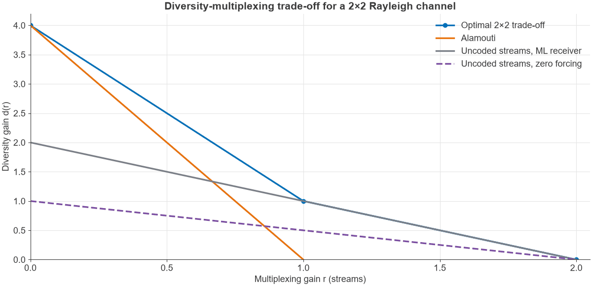
The trade-off has a formal statement due to Zheng and Tse. A scheme has multiplexing gain r if its rate grows as r log₂(SNR), and diversity gain d if its error rate falls as SNR^-d. For an N_t×N_r Rayleigh channel with long enough code blocks, the best possible d(r) is a piecewise linear curve joining (k, (N_t-k)(N_r-k)) for integer k. For 2×2 the corners are (0, 4), (1, 1) and (2, 0).

Figure 3 sets the fixed schemes against that limit. Alamouti achieves d(r) = 4(1 – r), which is optimal only at r = 0. Uncoded streams with an ML receiver achieve d(r) = 2 – r, and with zero forcing only 1 – r/2. ML streams follow the optimal curve only between r = 1 and r = 2, so neither fixed scheme covers it all. Coded schemes such as the Golden code are designed to follow the whole curve.

The curve is about high-SNR behaviour, so it says nothing about a specific SNR. Still, it is a clear statement of the rule that a link cannot have maximum rate and maximum reliability at once.

Switching between the modes: rank adaptation

Real links do not choose once. Cellular and Wi-Fi systems estimate the channel, then pick the number of layers (the rank) and the modulation for each scheduling interval. The receiver reports a recommended rank, or the transmitter infers it from channel reciprocity. Typically:

• At low SNR or high correlation, the link falls back to rank 1, with transmit diversity or beamforming.
• At high SNR with a well-conditioned channel, it uses as many streams as the channel supports.
• Hybrid automatic repeat request and coding add time and frequency diversity across both modes, which softens the penalty of multiplexing in fades.

Adaptation gets close to the better of the two curves at each SNR, as long as the CSI is fresh. This is how spatial multiplexing in 5G networks works in practice, with layers chosen per user.

Spatial multiplexing and beamforming

Beamforming is a third use of the same antennas. With transmit CSI, the transmitter steers power towards the receiver, which raises SNR through array gain instead of adding diversity or streams. The modes combine: MIMO precoding sends several streams along the strongest eigenmodes of the channel, so each stream has beamforming gain. In a 2×2 link, sending one stream on the top eigenmode is a form of beamforming, and sending two is closed-loop multiplexing. MU-MIMO applies the same idea with streams going to different users, covered in MIMO configurations.

RF design consequences

The two modes put different demands on hardware. Multiplexing at high order needs low error vector magnitude and low phase noise on every chain, because a residual error on one stream appears as interference on the other. Antenna correlation also matters more: at high correlation, the second singular value shrinks and the link loses rank, while Alamouti loses only part of its diversity. Diversity modes tolerate lower SNR and cheaper parts. See measuring radio performance for how EVM is checked and MIMO, beamforming and phased arrays for the architecture view.

Frequently asked questions

What is the difference between spatial diversity and spatial multiplexing?

Spatial diversity sends one data stream over several paths for reliability. Spatial multiplexing sends separate streams over those paths for a higher rate. On a 2×2 link at 20 dB, the second gives more on average, and the first gives more when 1% outage is the target.

Can a MIMO system use both at once?

Yes. A 4×4 link can send two streams, each protected by space-time coding across pairs of antennas. The trade-off curve shows that intermediate points exist, and practical systems choose among them with rank adaptation.

When should spatial multiplexing be turned off?

When SNR is low, antennas are highly correlated or the channel is close to pure line of sight with closely spaced antennas. In those conditions a rank 1 transmission delivers a better rate, because the second stream adds more interference than throughput.

Does spatial multiplexing need multipath?

Usually yes, because it needs the channel matrix to have more than one strong singular value. Well-spaced line-of-sight antennas can also provide this, as with point-to-point links covered in the spatial multiplexing article.

Related topics

The theory of streams is in spatial multiplexing in MIMO, and transmit and receive diversity covers the diversity side alone. Antenna counts are compared in SISO vs MIMO, and radio architectures shows how the chains are built.