

MIMO capacity is the highest error-free data rate a multi-antenna link can support, in bits per second per hertz, given its channel and SNR. For a channel matrix H with no channel knowledge at the transmitter, it is C = log2 det(I + (ρ/Nt) H HH). At high SNR it grows about min(Nt, Nr) times as fast as single-antenna capacity, and that factor is why multiple antennas raise throughput without extra bandwidth.
This article covers the capacity formula itself, the difference between ergodic and outage capacity, and the things that reduce capacity in practice, with curves computed from the formulas. MIMO and multiple antenna systems introduces the antenna configurations, and spatial multiplexing covers how a real link sends streams on these channels.
The MIMO capacity formula
Shannon capacity for a single antenna pair is log2(1 + ρ|h|2). The matrix version replaces the scalar gain with H. For Nt transmit and Nr receive antennas, equal power per antenna and total SNR ρ at each receive antenna:
C = log2 det(I + (ρ/Nt) H HH) b/s/Hz
The determinant hides a simple structure. If λi are the eigenvalues of H HH, which are the squared singular values of H, the formula becomes a sum over parallel channels:
C = Σi log2(1 + (ρ/Nt) λi)
Capacity therefore depends only on how the channel’s power is spread across its eigenvalues. A channel with several comparable eigenvalues beats one with the same total power concentrated in a single large eigenvalue, because the logarithm rewards spreading power.
Worked example: capacity of a 2×2 channel
Take H = [1, 0.5; 0.2, 1.2] at ρ = 10 (10 dB) in 20 MHz.
| Step | Result |
|---|---|
| Singular values of H | 1.474, 0.746 |
| Eigenvalues λ1, λ2 | 2.173, 0.557 |
| Condition number | 5.9 dB |
| Mode SNRs, (ρ/2)λi | 10.87, 2.78 |
| Mode rates | 3.569, 1.920 b/s/Hz |
| Capacity, equal power | 5.489 b/s/Hz (109.8 Mb/s) |
| Determinant form, as a check | 5.489 b/s/Hz |
| Capacity, water-filling | 5.506 b/s/Hz (110.1 Mb/s) |
| All power on the strongest mode | 4.507 b/s/Hz |
| AWGN SISO link at 10 dB, for reference | 3.459 b/s/Hz |
Both forms of the formula agree, and the weaker mode adds 1.92 b/s/Hz even though its eigenvalue is 3.9 times smaller. Sending all the power on the strong mode gives 4.507 b/s/Hz, which is 18% below capacity.
Ergodic capacity in Rayleigh fading
For a fading channel, H is random and capacity is a random variable. If coding spans many channel states, the achievable rate is the mean, called ergodic capacity. Figure 1 and the table use independent Rayleigh fading with no transmit CSI, averaged over 100,000 channels (40,000 for 8×8).
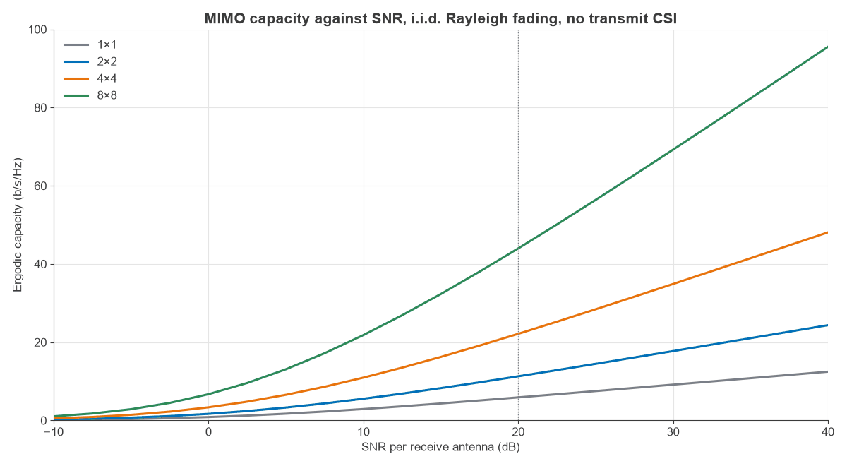
| SNR | 1×1 | 2×2 | 4×4 | 8×8 |
|---|---|---|---|---|
| 0 dB | 0.86 | 1.69 | 3.35 | 6.71 |
| 10 dB | 2.90 | 5.55 | 10.94 | 21.82 |
| 20 dB | 5.88 | 11.29 | 22.14 | 43.98 |
| 30 dB | 9.14 | 17.74 | 34.90 | 69.24 |
Values are in b/s/Hz. As a check, the exact 1×1 result e1/ρ E1(1/ρ) / ln 2 gives 0.860, 2.907 and 5.884 b/s/Hz at 0, 10 and 20 dB, against 0.86, 2.90 and 5.88 from simulation.
Multiplexing gain and the high-SNR slope
Between 30 and 40 dB, the curves rise by 1.00, 1.99, 3.97 and 7.91 b/s/Hz per 3 dB for 1×1, 2×2, 4×4 and 8×8. The slope is the multiplexing gain, min(Nt, Nr). At high SNR:
C ≈ min(Nt, Nr) log2(ρ) + constant
Each 3 dB of extra power therefore adds 1 b/s/Hz per spatial dimension. Capacity also scales almost linearly with antenna count at a fixed SNR: at 20 dB, 4×4 gives 3.77 times the 1×1 rate and 8×8 gives 7.48 times.
Outage capacity
Short blocks see one channel realisation, so the mean says little about a single transmission. Outage capacity Cε is the rate supported in all but a fraction ε of channel states. Figure 2 shows the distribution at 10 dB from 200,000 channels.
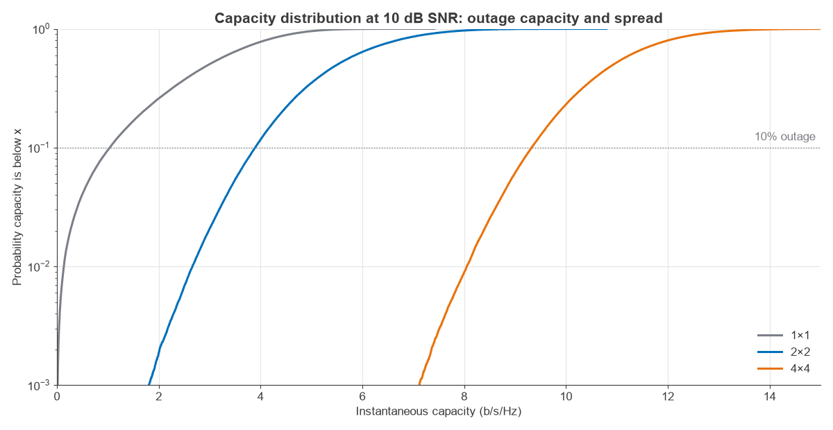
| Link at 10 dB | Mean (b/s/Hz) | Standard deviation | 10% outage | 1% outage | P(C below 8 b/s/Hz) |
|---|---|---|---|---|---|
| 1×1 | 2.90 | 1.31 | 1.03 | 0.14 | 100% |
| 2×2 | 5.55 | 1.31 | 3.89 | 2.65 | 96.7% |
| 4×4 | 10.94 | 1.27 | 9.32 | 8.06 | 0.87% |
The standard deviation stays close to 1.3 b/s/Hz as the mean rises, so the relative spread shrinks with antenna count. At 1×1 the 10% outage capacity is 36% of the mean, and at 4×4 it is 85%. This effect, called channel hardening, makes large MIMO links easier to schedule because the rate is more predictable. A fixed 8 b/s/Hz service is nearly impossible on 2×2 at this SNR and reliable on 4×4.
Effect of transmit CSI and water-filling
If the transmitter knows H, it can send along the eigenvectors and allocate power by water-filling:
Pi = max(μ − 1/λi, 0), with μ chosen so the powers sum to ρ
Strong modes get more power and very weak ones get none. Averaged over 40,000 4×4 Rayleigh channels:
| SNR | Equal power | Water-filling | Gain |
|---|---|---|---|
| −10 dB | 0.53 | 0.98 | 0.45 b/s/Hz (85%) |
| 0 dB | 3.35 | 4.21 | 0.86 b/s/Hz (26%) |
| 10 dB | 10.93 | 11.52 | 0.59 b/s/Hz (5.4%) |
| 20 dB | 22.12 | 22.26 | 0.14 b/s/Hz (0.6%) |
Transmit CSI is valuable at low SNR, where it concentrates power and adds array gain, and adds little at high SNR. The worked 2×2 channel shows the same thing: at 0 dB, water-filling raises capacity from 1.415 to 1.666 b/s/Hz by turning off the weak mode, while at 10 dB it adds only 0.017 b/s/Hz. Obtaining that CSI has a cost, which channel state information covers in detail.
Antenna correlation and channel capacity
Real antennas are not independent. Figure 3 uses a Kronecker model with exponential correlation, H = R1/2 G R1/2, where adjacent antennas at each end have correlation r and G is i.i.d. Rayleigh.
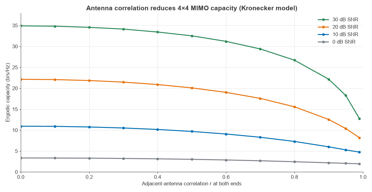
At 20 dB SNR, 4×4 capacity falls from 22.14 b/s/Hz at r = 0 to 21.45 at r = 0.3, 20.10 at r = 0.5, 17.57 at r = 0.7, 12.56 at r = 0.9 and 10.38 at r = 0.95. Moderate correlation costs little, and the loss accelerates beyond about 0.7. Capacity at r = 0.95 is 47% of the uncorrelated value, which is still above the 5.88 b/s/Hz of an uncorrelated SISO link at the same SNR. The Kronecker model is a simplification, since it assumes scattering at each end is independent of the other, but the trend is general. Antenna spacing and polarisation are the main ways to manage it, as antennas and propagation in radio design explains.
Capacity with more receive antennas than streams
Adding receive antennas beyond the transmit count does not raise the multiplexing gain, but it adds array gain. With Nt = 4 and Nr large, HHH/Nr tends to the identity, and capacity approaches:
C ≈ Nt log2(1 + ρ Nr/Nt)
| Antennas at 20 dB | Simulated | Large-Nr formula |
|---|---|---|
| 4×4 | 22.14 | 26.63 |
| 4×8 | 28.88 | 30.60 |
| 4×16 | 33.81 | 34.59 |
| 4×32 | 38.21 | 38.58 |
| 4×64 | 42.39 | 42.58 |
Each doubling past 4×16 adds about 4.3 b/s/Hz, close to the 4 b/s/Hz expected from 1 b/s/Hz per stream for each 3 dB of array gain. This is the single-cell basis of massive MIMO. The formula is poor at 4×4, where H is nearly singular in many draws, and very close at 4×64.
From capacity to real throughput
Capacity is a bound, and a real link falls short in several ways. Practical coding sits some way from the bound, by anything from a fraction of a dB to a few dB. Pilots and control signals use up resource elements. Channel estimates contain errors, transmitters add error vector magnitude, and linear receivers fall below capacity, as the MIMO detection algorithms page shows. Interference from other cells also lowers the effective SNR, which is the subject of MIMO interference management.
The formula still gives useful estimates. To compare two antenna configurations, take the SNR from a link budget, read the capacity from Figure 1 and apply the same fractional loss to both.
Frequently asked questions
How do you calculate MIMO capacity?
Find the eigenvalues λi of H HH, then sum log2(1 + (ρ/Nt) λi). Multiply by bandwidth for a rate in bits per second. For a fading channel, average this over many channel draws to get ergodic capacity.
Does MIMO capacity increase linearly with antennas?
It increases about linearly with min(Nt, Nr) in rich scattering, as the 20 dB row shows. Adding antennas at one end only gives logarithmic growth, because the extra antennas add array gain and not spatial dimensions.
What is the difference between ergodic and outage capacity?
Ergodic capacity is the mean over channel states and applies when coding spans many of them. Outage capacity is the rate available with a stated reliability on a single state. It suits delay-limited traffic, and it is always below the mean at low outage probabilities.
Does MIMO capacity need multipath?
In a typical non-line-of-sight link, multipath supplies the independent eigenvalues. A pure line-of-sight channel normally has rank 1, but carefully spaced antennas can create rank above 1 without multipath, a case covered under spatial multiplexing.
Related topics
Capacity sets the limit for spatial multiplexing, while beamforming uses antennas for gain and MIMO precoding uses transmit CSI to approach the bound. For hardware that determines how close a design can get, see MIMO, beamforming and phased-array architectures and measuring radio performance. The broader picture is in RF design.