


Antenna diversity in a SIMO or MISO link comes down to one choice: how to use the extra antennas at the end of the link that has them. SIMO receivers choose between selection, equal gain and maximal ratio combining, while MISO transmitters choose between antenna selection, channel-matched beamforming and space-time coding. The best choice depends on branch balance, correlation and how fresh the channel information is.
This article compares those diversity techniques with numbers, so that a designer can decide which one earns its hardware. What diversity is and how it reduces fades is in transmit and receive diversity, and the difference between the configurations is in SISO vs MIMO.
Antenna diversity in SIMO and MISO links
A SIMO link (one transmit antenna, several receive antennas) sees channel vector h at the receiver, so all the processing sits there. A MISO link (several transmit antennas, one receive antenna) sees the same vector from the other side, but the transmitter must act before the signal has passed through the channel. It can only do so with channel state information (CSI) fed back or inferred. Each SIMO method has a MISO counterpart:
| SIMO receiver method | MISO transmitter counterpart | Transmit CSI needed |
|---|---|---|
| Selection combining (SC) | Transmit antenna selection (TAS) | Best antenna index only |
| Equal gain combining (EGC) | Equal gain transmission | Phases |
| Maximal ratio combining (MRC) | Maximum ratio transmission (MRT) | Phases and amplitudes |
| No direct counterpart | Alamouti space-time code | None |
SIMO diversity combining methods
With L branches and branch signals hk, the three standard receivers differ in what they do with the amplitude and phase of each branch.
- Selection combining takes the strongest branch. Output SNR is the maximum of the branch SNRs. It can use one receive chain and an RF switch, which is why it suits low-cost radios, though the switch adds a little loss ahead of the noise figure budget.
- Equal gain combining aligns phases and adds branches with equal weights. Output SNR is (Σ|hk|)2/L times the mean branch SNR. It needs no amplitude estimate.
- Maximal ratio combining weights each branch by the conjugate of its channel. Output SNR is the sum of the branch SNRs, the highest of any linear combiner when noise is equal and independent across branches. It needs a complete chain and a channel estimate per branch.
Mean SNR gain
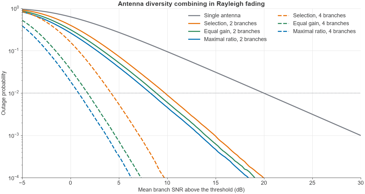
The mean SNR rises by HL = Σk=1..L 1/k for selection, 1 + (L-1)π/4 for EGC in Rayleigh fading, and L for MRC. The mean gain columns of the next table use these formulas. A simulation of 2 million Rayleigh draws matched each to within 0.1%.
Gain at low outage
Mean SNR understates diversity, because the benefit is at the bottom of the distribution. The table gives both measures, with the reduction in mean SNR needed for a fixed 1% outage compared with one antenna.
| Branches | SC mean gain | SC at 1% outage | EGC mean gain | EGC at 1% outage | MRC mean gain | MRC at 1% outage |
|---|---|---|---|---|---|---|
| 2 | 1.76 dB | 10.2 dB | 2.52 dB | 11.1 dB | 3.01 dB | 11.7 dB |
| 3 | 2.63 dB | 13.8 dB | 4.10 dB | 15.6 dB | 4.77 dB | 16.4 dB |
| 4 | 3.19 dB | 15.8 dB | 5.26 dB | 18.2 dB | 6.02 dB | 19.1 dB |
Two results stand out. First, most of the benefit arrives with the second antenna, whichever method is used. Second, EGC sits close to MRC, within 0.6 dB for two branches and 0.9 dB for four, so a design that cannot estimate amplitude well gives up little. Selection falls behind as L grows, since it discards the other branches: the shortfall against MRC rises from 1.5 dB at L = 2 to 3.3 dB at L = 4.
Worked example: combiner choice at 2 branches
A receiver needs 5 dB SNR and sees a mean of 15 dB on each branch, so x = 10-1 = 0.1. The outage probabilities are:
- Single antenna: 1 – e-0.1 = 0.0952
- Selection: (1 – e-0.1)2 = 0.00906
- Equal gain: 0.00616 (numerical integration)
- Maximal ratio: 1 – e-0.1(1.1) = 0.00468
Turning this around, the mean branch SNR needed for 1% outage at the same 5 dB threshold is 25.0 dB with one antenna, 14.8 dB with selection, 13.9 dB with EGC and 13.3 dB with MRC. The step from one antenna to selection saves 10.2 dB. The step from selection to MRC saves 1.5 dB, at the price of a second receive chain. For a battery-powered receiver, that comparison often favours selection.
Antenna diversity selection: when branches are not equal
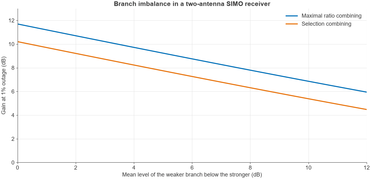
The tables above assume equal, independent branches. Real antennas differ. A phone held in the hand, or a dual-polarised antenna on a mainly co-polar path, can leave one branch well below the other.
Branch imbalance
For two independent branches with mean powers Γ1 and Γ2, MRC outage is 1 – (Γ1e-x/Γ1 – Γ2e-x/Γ2)/(Γ1 – Γ2), and selection outage is the product (1 – e-x/Γ1)(1 – e-x/Γ2).
| Weaker branch | MRC gain at 1% outage | SC gain at 1% outage |
|---|---|---|
| Equal | 11.7 dB | 10.2 dB |
| 3 dB down | 10.2 dB | 8.7 dB |
| 6 dB down | 8.8 dB | 7.3 dB |
| 10 dB down | 6.9 dB | 5.4 dB |
Each decibel of imbalance costs roughly half a decibel of gain. The diversity survives well: a branch 10 dB down still saves 6.9 dB at 1% outage, so the second antenna need not be as good as the first. The gap between MRC and selection stays near 1.5 dB throughout.
Branch correlation
Correlation behaves similarly. At an envelope correlation of 0.5, two-branch gain at 1% outage falls to 10.3 dB for MRC, 9.7 dB for EGC and 8.8 dB for selection. At 0.9 they are 7.2, 6.6 and 5.7 dB. The method does not change the ranking, and the spacing needed to reach low correlation is worked out in diversity techniques in wireless communication.
MISO diversity and channel feedback
MISO adds a constraint that SIMO lacks. Total power is fixed, and the transmitter must know the channel. With perfect CSI and equal total power, MRT matches MRC at 11.7 dB for two antennas and TAS matches selection at 10.2 dB. Alamouti needs no transmit CSI, but it shares power between antennas, so it gains 3.01 dB less than MRC: 8.7 dB at 1% outage.
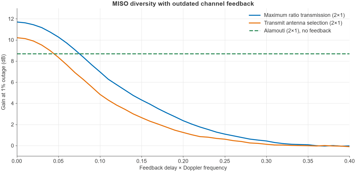
In practice CSI is old by the time it is used. If the channel changes with Clarke statistics, the correlation between the channel used and the channel seen after delay τ is ρ = J0(2πfdτ). Figure 3 plots the resulting gain from a simulation, with Alamouti as a flat reference.
Worked example: feedback delay at 3.5 GHz
A 3.5 GHz device moving at 3 km/h has a Doppler shift close to 10 Hz. With a feedback delay of 10 ms, fdτ = 0.1 and ρ = J0(0.628) = 0.904.
- Mean gain of two-antenna MRT falls from 3.01 dB to 2.59 dB, from 1 + ρ2 = 1.82.
- MRT gain at 1% outage falls from 11.7 dB to 7.0 dB.
- TAS gain at 1% outage falls from 10.2 dB to 4.9 dB.
- Alamouti stays at 8.7 dB, because it uses no feedback.
The mean hardly moves, yet much of the deep-fade protection has gone. With 5 ms delay at 5 Hz Doppler (fdτ = 0.025), MRT still gives 11.3 dB and beats Alamouti. Figure 3 puts the crossover near fdτ = 0.075 for MRT and 0.045 for TAS. Above those values, open-loop coding protects better than closed-loop feedback. A related point is that channel state information feedback also costs overhead, which grows with antenna count.
Choosing a diversity technique
- Cost-driven SIMO receiver: selection with an RF switch, where the extra 1.5 dB of MRC does not justify a second chain.
- Receiver with chains already present: MRC. If a MIMO radio already has the chains, it costs little more than software.
- Poor amplitude estimates: EGC, within about 0.6 dB of MRC at two branches.
- MISO with slow-moving users and short feedback delay: MRT, for the full 3 dB of array gain.
- MISO with fast users or no feedback: Alamouti or other open-loop transmit diversity.
- MISO with one RF chain: TAS, ideally with low feedback delay.
Frequently asked questions
What is antenna diversity selection?
It is the simplest form of antenna diversity. The radio measures each antenna and uses the strongest, by switching one receive chain between antennas. It delivers most of the available gain, 10.2 dB of a possible 11.7 dB at 1% outage for two branches.
Is MRC always better than selection combining?
For equal noise across branches and accurate channel estimates, yes, because MRC uses all branches. If channel estimates are noisy or a second chain would add cost and power, selection may be the better engineering choice, since the difference is only about 1.5 dB at two branches.
How does MIMO diversity relate to SIMO and MISO diversity?
MIMO can use both. With a single stream, a 2×2 link can reach diversity order 4, combining transmit and receive techniques. Adding streams uses up some of that diversity, a trade-off covered in spatial diversity and spatial multiplexing.
Does transmit diversity work as well as receive diversity?
Not without transmit CSI. Alamouti has the same diversity order as two-branch MRC, but it is 3.01 dB worse because the transmitter divides a fixed power and the receiver has no array gain. With fresh CSI, MRT matches MRC.
Related topics
SIMO vs MIMO looks at when to add transmit antennas as well, and MIMO and multiple antenna systems gives the wider picture of array gain and capacity. Link budget use of these gains is in the RF link budget guide, and antenna background is in the antennas hub.