

Spatial multiplexing sends independent data streams from different antennas in the same frequency band and at the same time, and the receiver separates them using the differences in their spatial signatures. The number of streams cannot exceed the rank of the MIMO channel, which is at most the smaller of the transmit and receive antenna counts. In a well-conditioned channel at high SNR, capacity then grows about linearly with that number, with no added bandwidth or transmit power.
This is the rate-raising use of a MIMO and multiple antenna system. The alternative, beamforming, spends the same antennas on power gain. The RF hardware that supports both is described in MIMO, Beamforming and Phased-Array Architectures.
The MIMO channel model
With Nt transmit and Nr receive antennas, a narrowband channel is written as:
y = Hx + n
Here H is an Nr x Nt complex matrix and entry hij is the gain from transmit antenna j to receive antenna i. In a wideband OFDM system this model applies to each subcarrier.
SVD, rank and parallel channels
The singular value decomposition H = UΣVH explains spatial multiplexing. If the transmitter precodes with V and the receiver multiplies by UH, the channel becomes a set of independent parallel pipes with gains σi, the singular values of H. With equal power per stream and total SNR ρ, capacity is:
C = Σi log2(1 + (ρ/Nt) σi2) b/s/Hz
The rank of H is the number of non-zero singular values. In practice, what counts is how many are large enough to carry useful SNR. The condition number, σmax/σmin, is the usual measure of this, and it is often quoted in dB as 20 log10 of that ratio.
Worked example: two 2×2 channels
The comparison below uses two real 2×2 channels with nearly the same total power gain, so that only their structure differs. The SNR is 20 dB (ρ = 100), and rates are given for 100 MHz of bandwidth.
Channel A is HA = [1, 1; 1, -1]. Channel B is HB = [1.2, 0.75; 0.75, 1.2].
| Quantity | Channel A | Channel B |
|---|---|---|
| Sum of |hij|2 | 4.000 | 4.005 |
| Singular values | 1.414, 1.414 | 1.950, 0.450 |
| Condition number | 1.00 (0.0 dB) | 4.33 (12.7 dB) |
| Stream SNRs, (ρ/2)σi2 | 20.0 dB, 20.0 dB | 22.8 dB, 10.1 dB |
| Stream rates (b/s/Hz) | 6.66, 6.66 | 7.58, 3.48 |
| Capacity, equal power | 13.32 b/s/Hz | 11.05 b/s/Hz |
| Rate in 100 MHz | 1,332 Mb/s | 1,105 Mb/s |
| Capacity, water-filling | 13.32 b/s/Hz | 11.06 b/s/Hz |
| Zero-forcing SINR per stream | 20.0 dB | 12.8 dB |
| Zero-forcing sum rate | 13.32 b/s/Hz | 8.68 b/s/Hz |
| Single stream, all power on σmax | 7.65 b/s/Hz | 8.57 b/s/Hz |
Three results stand out. Channel B loses 17% of its capacity to poor conditioning, even though it carries the same total power gain. Water-filling hardly helps at this SNR, adding only 0.003 b/s/Hz with a 52/48 power split. The largest effect is on the receiver: zero forcing cuts channel B to 8.68 b/s/Hz, little more than the 8.57 b/s/Hz available from sending a single stream.
Receivers for spatial multiplexing
Without precoding, each receive antenna sees a mixture of all the streams, and the receiver must unmix them. The main options differ in performance and complexity.
- Zero forcing (ZF) applies the pseudo-inverse of H. It removes inter-stream interference completely, but amplifies noise along weak directions, so its SINR on stream k is (ρ/Nt) / [(HHH)-1]kk.
- Linear MMSE balances interference against noise. It approaches ZF at high SNR and is noticeably better at low SNR.
- Successive interference cancellation (SIC) decodes one stream, subtracts it and moves on. With MMSE filtering and ideal rate control per stream it can reach capacity, though errors can propagate between stages.
- Maximum likelihood searches all MNs symbol combinations. For four streams of 64-QAM that is 644, or about 16.8 million candidates per symbol, so sphere decoders and list methods are used to approximate it.
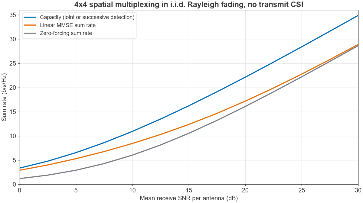
For an i.i.d. Rayleigh 4×4 channel with no transmit CSI, Monte Carlo averaging over 60,000 channels gives these sum rates:
| SNR | Capacity | Linear MMSE | Zero forcing |
|---|---|---|---|
| 10 dB | 10.94 b/s/Hz | 8.44 b/s/Hz | 6.04 b/s/Hz |
| 20 dB | 22.13 b/s/Hz | 17.18 b/s/Hz | 16.08 b/s/Hz |
Figure 1 shows the full range. The curves share a slope at high SNR, close to 4 b/s/Hz per 3 dB (a 30 to 33 dB step gives 3.94 b/s/Hz), so linear receivers keep the multiplexing gain and lose a fixed SNR offset.
Open-loop and closed-loop operation
Open-loop spatial multiplexing sends streams with no knowledge of H at the transmitter, and relies on the receiver alone to separate them. Closed-loop operation uses CSI, either fed back or inferred from channel reciprocity in TDD, to precode. Feedback is often quantised into a codebook index, which saves overhead but limits accuracy.
A frequent source of confusion concerns space-time codes. Alamouti coding sends one symbol per use of the channel across two antennas, so it is a diversity technique and carries no multiplexing gain. In this context “SM” can also mean spatial modulation, a different scheme that activates only some antennas at a time.
Rank adaptation and when not to multiplex
Spatial multiplexing is not always the best choice. For a 4×4 Rayleigh channel, the comparison between sending four equal-power streams and sending all power on the strongest eigenmode (which needs CSI at the transmitter) is:
| SNR | Four streams, no CSI | One stream on dominant eigenmode |
|---|---|---|
| 0 dB | 3.35 b/s/Hz | 3.38 b/s/Hz |
| 20 dB | 22.13 b/s/Hz | 9.88 b/s/Hz |
At 0 dB the two are about equal, and the single stream needs far less decoding effort. At 20 dB multiplexing more than doubles the rate. Systems therefore adapt the rank alongside the modulation and coding, using channel quality reports to pick the number of streams on each scheduling interval. Multi-user MIMO applies the same idea to several devices at once, which suits a base station with many antennas serving handsets with few.
Antenna correlation
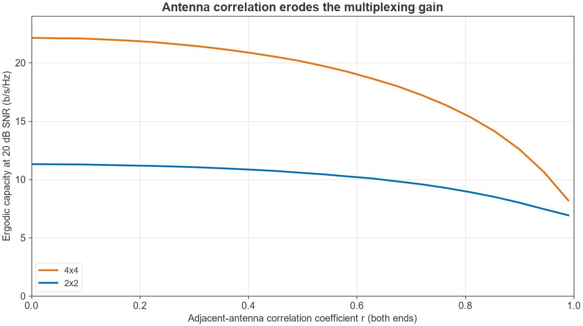
Correlation between antennas pulls the singular values apart. Using a Kronecker model, with exponential correlation r|i-j| at both ends, ergodic capacity at 20 dB SNR falls as follows:
| Correlation r | 4×4 capacity (b/s/Hz) | 2×2 capacity (b/s/Hz) |
|---|---|---|
| 0 | 22.1 | 11.3 |
| 0.5 | 20.1 | 10.6 |
| 0.7 | 17.6 | 9.7 |
| 0.9 | 12.6 | 8.0 |
| 0.95 | 10.4 | 7.4 |
Moderate correlation does little damage, but the loss is steep above about 0.7. Figure 2 shows the shape of this. Spacing and polarisation diversity, covered in the multiple antennas overview, are the main design tools for avoiding it. Dual polarisation is especially useful, because it provides two low-correlation streams in one aperture.
Line-of-sight MIMO
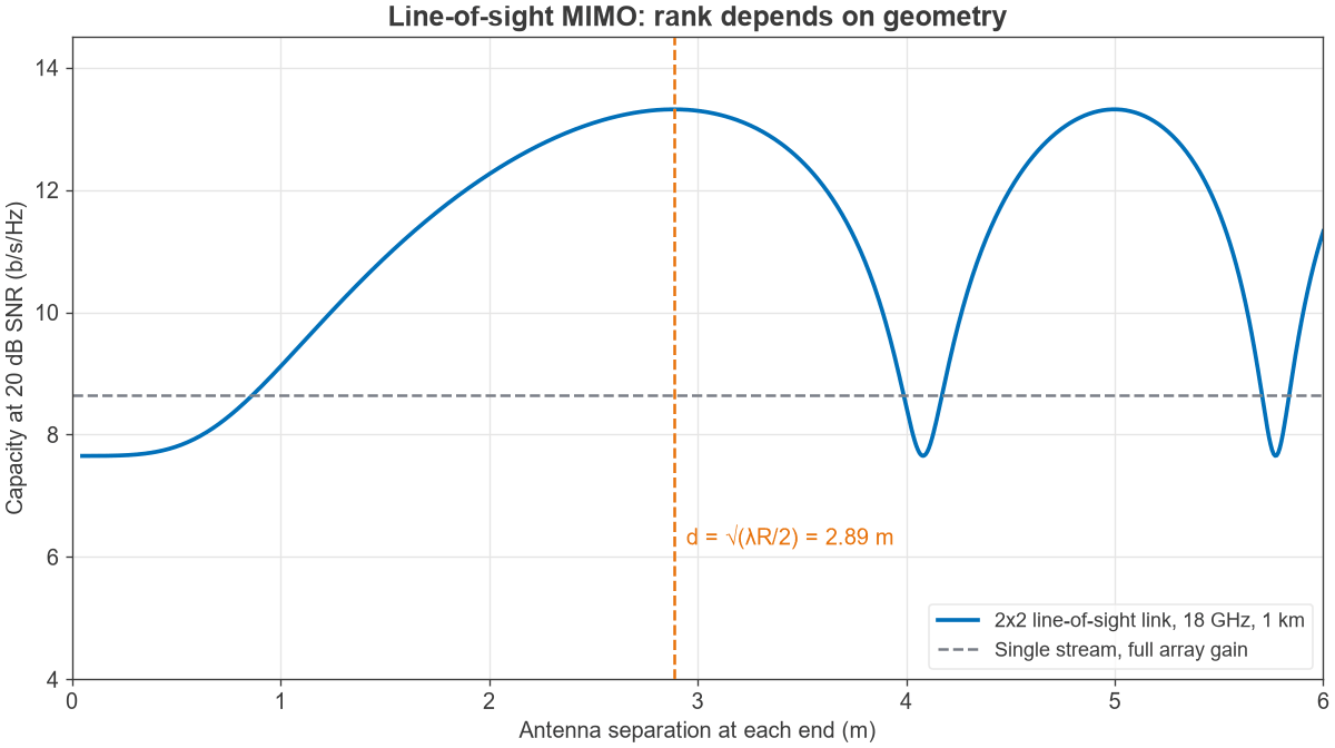
Multiplexing does not strictly need multipath. If antennas are spaced widely enough, a pure line-of-sight channel can have full rank, because spherical wavefronts produce different phases across the array. For two parallel two-element arrays at range R, with separation d at each end, the channel is orthogonal when:
d = √(λR/N), which for N = 2 is √(λR/2)
Worked example: an 18 GHz point-to-point link
At 18 GHz, λ = 16.66 mm. Over R = 1 km, the required separation is 2.89 m at each end. The table shows capacity at 20 dB SNR with power equally divided.
| Separation | Singular values | Capacity (b/s/Hz) |
|---|---|---|
| 0.2 m | 2.000, 0.008 | 7.66 |
| 0.5 m | 1.999, 0.047 | 7.80 |
| 1.0 m | 1.991, 0.188 | 9.11 |
| 2.89 m | 1.414, 1.414 | 13.32 |
At 2.89 m this gives the same result as channel A above, and at small separations it behaves as a rank-1 link. Figure 3 also shows the single-stream reference of 8.65 b/s/Hz, which assumes all power on the single mode. The link is sensitive to geometry, since the curve repeats and falls back to rank 1 at certain larger separations, and the optimum moves with range and frequency. Applications are mostly fixed links, since mobile channels rarely offer this geometry.
RF requirements for multiplexing
High-order streams depend on the transmitter’s error vector magnitude. Impairments such as PA compression, phase noise and IQ imbalance act like added noise, placing a ceiling on SINR. As a simple approximation, with EVM treated as noise-like:
SINR ≈ 1 / (1/SNR + EVM2)
Taking four streams at a 30 dB channel SNR (ideal total 39.9 b/s/Hz):
| EVM | SINR per stream | Sum rate (b/s/Hz) |
|---|---|---|
| -40 dB | 29.6 dB | 39.3 |
| -30 dB | 27.0 dB | 35.9 |
| -25 dB | 23.8 dB | 31.7 |
| -20 dB | 19.6 dB | 26.1 |
Each stream must meet this budget at the same time, and PAPR forces the PAs into back-off. See Modulation, EVM and PAPR for how that budget is built. Isolation between chains also matters: leakage at the transmitter adds to the mixing that the receiver has to undo, and it looks like a worse channel. Testing these effects is covered under measuring radio performance.
Frequently asked questions
How many spatial streams can a link support?
At most min(Nt, Nr), and often fewer. The usable count depends on the rank of the channel and on SNR. A handset with two or four antennas limits a link regardless of the base station’s size, and systems report and adapt rank continuously.
Does spatial multiplexing need multipath?
It needs a channel with several strong singular values, and multipath is the usual source. Dual polarisation can provide two streams with little scattering, and carefully spaced line-of-sight arrays provide rank by geometry. A narrow line-of-sight channel with close spacing supports one stream.
What is the difference between spatial multiplexing and spatial diversity?
Multiplexing sends different data on each stream, raising the rate. Diversity sends related copies of the same data, reducing fades. A link can trade between the two, and adaptive systems move between them according to SNR and channel conditions.
Why does a high condition number hurt?
A high condition number means one spatial direction is much weaker than the others. Linear receivers amplify noise along that direction to recover the stream, and the SINR falls for every stream carried on it. In the worked example, zero forcing lost over 7 dB in this way.
Related topics
The multiple antennas overview sets this topic alongside array gain and diversity, and beamforming covers the use of the same antennas for power gain. MIMO, Beamforming and Phased-Array Architectures describes the radio design, and the link budget article shows how required SNR is set.