


Interference cancellation removes an unwanted signal after it has reached the receiver, by estimating that signal, reconstructing it and subtracting it. In MIMO systems it takes two main forms: digital cancellation of other data streams, as in successive and parallel interference cancellation, and RF interference cancellation of a strong known signal before the receiver saturates, as in full-duplex radios. In each form, the depth is set by how accurately the replica matches the real interferer.
This page is about that subtraction and its limits. It applies to a radio that already has the interference at its input. Stopping the interference at its source is a different job, covered in interference avoidance and mitigation, and MIMO interference management compares all the options.
How interference cancellation works
An interfering signal i(t) arrives through a channel h, so the receiver sees the wanted signal plus h·i(t). If the receiver has an estimate î of the signal and an estimate ĥ of the channel, it forms the replica ĥ·î and subtracts it. Whatever survives is the residual:
residual = h·i − ĥ·î
Cancellation differs from suppression in one respect. Interference suppression, such as an MMSE or interference rejection receiver, applies a spatial filter that projects the interferer away, and uses up a receive dimension in doing so. Cancellation reconstructs the interferer and removes it, so the wanted signal keeps all its dimensions. The price is that cancellation needs to know the interfering waveform, either because it is the radio’s own transmission or because it has been decoded.
Interference cancellation depth
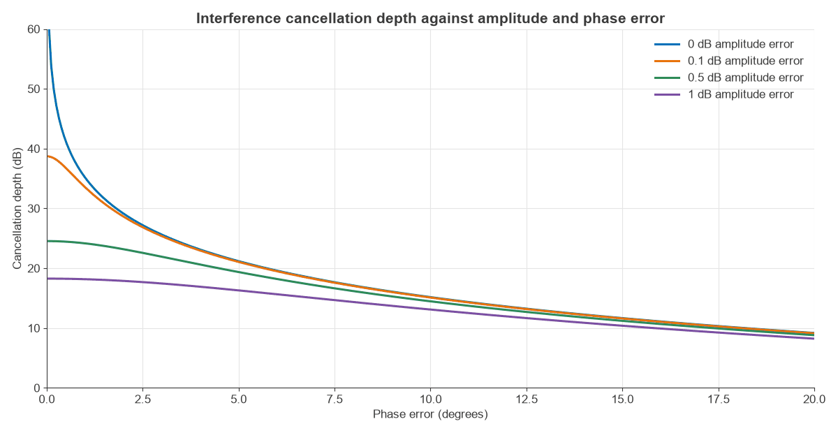
Depth is the ratio of interferer power before and after subtraction. If the replica has amplitude ratio a and phase error φ relative to the true signal:
D = 1 / |1 − a ejφ|2
| Amplitude error | Phase error | Depth |
|---|---|---|
| 0.1 dB | 0 | 38.7 dB |
| 1 dB | 0 | 18.3 dB |
| 0 | 1° | 35.2 dB |
| 0 | 10° | 15.2 dB |
| 0.1 dB | 1° | 33.5 dB |
| 0.5 dB | 5° | 19.4 dB |
| 1 dB | 10° | 13.1 dB |
The amplitude errors in the table have the replica too large, which is the worse sign: a replica 1 dB too small gives 19.3 dB. As a rule of thumb, 1° of phase error caps depth near 35 dB and 0.1 dB of amplitude error near 39 dB. Deep cancellation is a matching exercise. A 40 dB canceller needs its replica matched to about 1% in voltage, which is a demanding requirement to hold over temperature and frequency.
Broadband interference cancellation
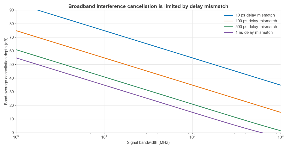
A single amplitude and phase setting can only match at one frequency. If the replica path differs from the true path by a delay Δτ, the phase error varies across the band. Averaged over bandwidth B:
D = 1 / [2(1 − sinc(BΔτ))], with sinc(x) = sin(πx)/(πx)
For small BΔτ this falls by 20 dB per decade of bandwidth or delay. Figure 2 plots it.
| Bandwidth | 100 ps mismatch | 500 ps mismatch | 1 ns mismatch |
|---|---|---|---|
| 20 MHz | 48.8 dB | 34.8 dB | 28.8 dB |
| 100 MHz | 34.8 dB | 20.9 dB | 14.8 dB |
| 400 MHz | 22.8 dB | 8.9 dB | 3.1 dB |
Depth at the band edge is about 4.8 dB worse than the average in each case (34.8 dB falls to 30.1 dB at 100 MHz with 100 ps). For scale, 100 ps is about 2 cm of coaxial cable, so physical layout decides the result. Broadband cancellers therefore use several delayed taps whose weights form a filter that matches the true response across the band, in the same way as an adaptive equaliser. The real leakage path also contains reflections from the antenna and nearby objects, so a tap count that works on the bench may fall short in the field.
RF interference cancellation for full-duplex MIMO
An interference cancellation radio that transmits and receives on one frequency must remove its own transmit signal, which is by far the strongest thing at its input. Take a 23 dBm transmitter with 100 MHz of bandwidth and a 6 dB receiver noise figure. The noise floor is −174 + 80 + 6 = −88 dBm, so the required self-interference cancellation is 23 − (−88) = 111 dB.
No single stage provides this, so the budget is spread:
| Stage | Reduction | Level after stage |
|---|---|---|
| Transmit power | None | +23 dBm |
| Antenna isolation | 30 dB | −7 dBm |
| Analog RF canceller | 40 dB | −47 dBm |
| Digital cancellation | 41 dB | −88 dBm |
The order is forced by the ADC. A 12-bit converter has about 74 dB of ideal dynamic range, or roughly 64 dB after a 10 dB allowance for signal peaks. At −47 dBm, the residual sits 41 dB above noise, leaving about 23 dB of margin. Without analog cancellation, the residual at the ADC would be far beyond that range, and digital processing could not recover what the converter never resolved.
Digital cancellation also has a blind spot. The baseband only knows the ideal transmit samples, not the noise and distortion added by the PA and oscillator. If transmit EVM is −40 dB, that unknown component is at 23 − 40 = −17 dBm, and after 70 dB of isolation and analog cancellation it is at −87 dBm. That is 1 dB above the noise floor, raising it by 3.5 dB. The usual remedies are to take the analog reference after the PA, so that it includes those impairments, or to model the non-linearity in the digital canceller. In a MIMO radio, each receive chain must also cancel every transmit chain, so the number of cancellation paths grows as NtNr: four paths for 2×2 and sixteen for 4×4.
Successive interference cancellation
Digital interference cancellation works on signals the radio did not transmit, by decoding them first. In successive interference cancellation (SIC), the receiver decodes the strongest signal, subtracts it and moves to the next one. It suits very unequal power levels, as in power-domain non-orthogonal access and in the strong-interference regime.
The residual now comes from channel estimate error. Worked example: a strong signal at 35 dB and a weak one at 15 dB above noise share a receiver.
| Quantity | Result |
|---|---|
| Strong signal SINR, weak treated as noise | 19.9 dB (6.61 b/s/Hz) |
| Weak signal rate with perfect cancellation | 15.0 dB (5.03 b/s/Hz) |
| Channel NMSE −25 dB: residual 10 dB above noise | SINR 4.6 dB (1.95 b/s/Hz) |
| Channel NMSE −35 dB: residual at noise level | SINR 12.0 dB (4.07 b/s/Hz) |
Estimate quality matters more as the power gap widens, because the residual scales with the strong signal. Here, a 10 dB better channel estimate doubles the weak user’s rate.
Parallel interference cancellation
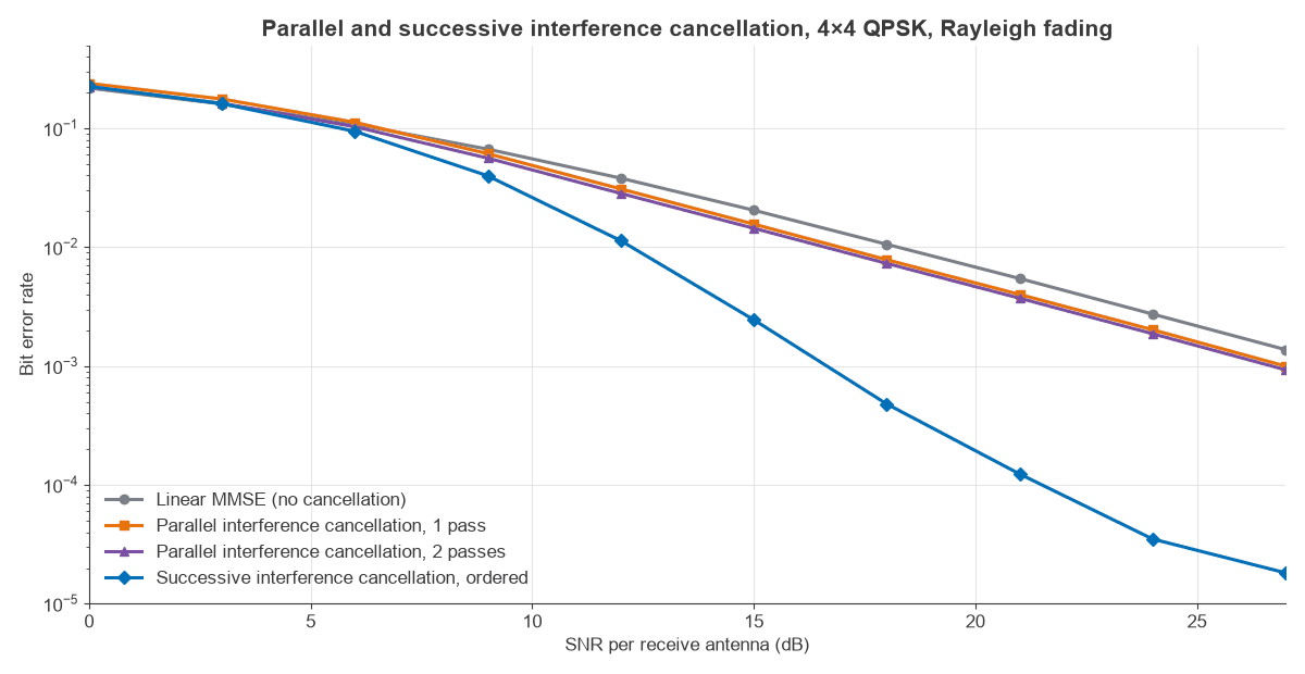
Parallel interference cancellation (PIC) estimates all streams at once, then subtracts all others from each one, and can repeat that process. It takes fewer stages than SIC and suits parallel hardware, and it is less exposed to one bad early decision. Figure 3 compares hard-decision PIC after an MMSE first stage with ordered MMSE-SIC, for uncoded 4×4 QPSK in Rayleigh fading over 9.6 million bits per point.
| Detector | SNR at BER 10−2 | BER at 24 dB, perfect CSI | BER at 24 dB, −20 dB NMSE |
|---|---|---|---|
| Linear MMSE | 18.3 dB | 2.7×10⁻³ | 1.3×10⁻² |
| PIC, 1 pass | 16.9 dB | 2.0×10⁻³ | 8.2×10⁻³ |
| PIC, 2 passes | 16.6 dB | 1.9×10⁻³ | 7.7×10⁻³ |
| Ordered SIC | 12.3 dB | 3.5×10⁻⁵ | 8.1×10⁻⁴ |
Hard-decision PIC gains only about 1.7 dB here, because the first stage fails in the same deep fades where PIC most needs good decisions, and a second pass adds little. Ordered SIC gains about 6 dB. That result applies to uncoded hard decisions. Soft PIC inside a turbo loop, where the subtraction is weighted by the decoder’s confidence, performs far better and is the usual form in coded receivers. With channel error, each scheme’s BER rises sharply and the SIC curve flattens at high SNR. A full comparison of detection methods is on the MIMO detection algorithms page.
Interference cancellation in massive MIMO
With many antennas per user, linear processing removes most inter-user interference, so subtraction is less necessary at the base station. It still has a role against pilot-contaminated signals and in dense uplinks, where SIC after zero forcing or MMSE can recover the last few dB. In all these cases the channel estimate sets the limit, in the same way as it does for an analog canceller’s replica.
Frequently asked questions
What is interference cancellation?
It is a technique that estimates an unwanted signal and subtracts it from the received signal, leaving the wanted signal. It can be done in RF, in baseband or across data streams after decoding. The limit is how closely the reconstructed signal matches the real one.
What is the difference between interference cancellation and interference suppression?
Suppression filters the interferer out, using spatial or frequency selectivity, and costs a degree of freedom. Cancellation reconstructs the interferer and subtracts it, and that needs knowledge of the waveform. Receivers often combine both.
How much RF interference cancellation is needed for full duplex?
About the transmit power minus the receiver noise floor. For 23 dBm and a −88 dBm noise floor that is 111 dB, split between antenna isolation, analog RF cancellation and digital cancellation. Lower power or narrower bandwidth changes that figure directly.
What limits broadband interference cancellation?
Delay mismatch and frequency-dependent paths. A single path with 100 ps mismatch gives about 35 dB across 100 MHz and only 23 dB across 400 MHz. Multi-tap cancellers improve this, but they must track reflections that change with the environment.
Related topics
For the wider picture, see MIMO interference management and interference avoidance and mitigation. Spatial alternatives are covered in beamforming and MIMO precoding. Receiver limits follow from noise figure and radio architectures, and the transmitter side from modulation, EVM and PAPR.