


Interference mitigation in MIMO systems covers every method of limiting unwanted signals, and interference avoidance is the part that stops them reaching a receiver in the first place. Avoidance works before transmission, by choosing when, where, in which direction and at what frequency and power to send, so that the receiver has little to deal with. It costs resources such as spectrum, antenna dimensions or channel knowledge, but it does not need the receiver to do anything.
This article looks at avoidance from the transmitter’s and the planner’s side. Once interference has arrived, the tools are different, and interference cancellation in MIMO systems covers those. MIMO interference management compares both approaches on one scenario.
Interference avoidance and interference mitigation
The terms are often mixed, so it helps to separate them by when each one acts.
| Stage | Example techniques | Who acts |
|---|---|---|
| Before transmission: avoidance | Frequency reuse, scheduling, transmit nulling, power control, listen before talk | Transmitter, network, planner |
| During reception: suppression | Directional receive beams, MMSE and IRC receivers, filtering | Receiver |
| After reception: cancellation | SIC, PIC, self-interference cancellation | Receiver |
Interference mitigation is the umbrella term for all three rows. A sound design generally starts at the top. Each dB that avoidance prevents is a dB the receiver does not have to handle, and a receiver’s ability to deal with interference is limited by its dynamic range and spatial dimensions. Avoidance is often a cheaper way to protect a victim that has only one antenna or that cannot be upgraded.
Interference avoidance in frequency: reuse planning
The oldest interference avoidance technology is keeping co-channel transmitters apart. Dividing spectrum among K cells in a cluster moves the nearest co-channel cell further away, to a distance of about √(3K) cell radii in a hexagonal layout, at the cost of each cell using only 1/K of the band.
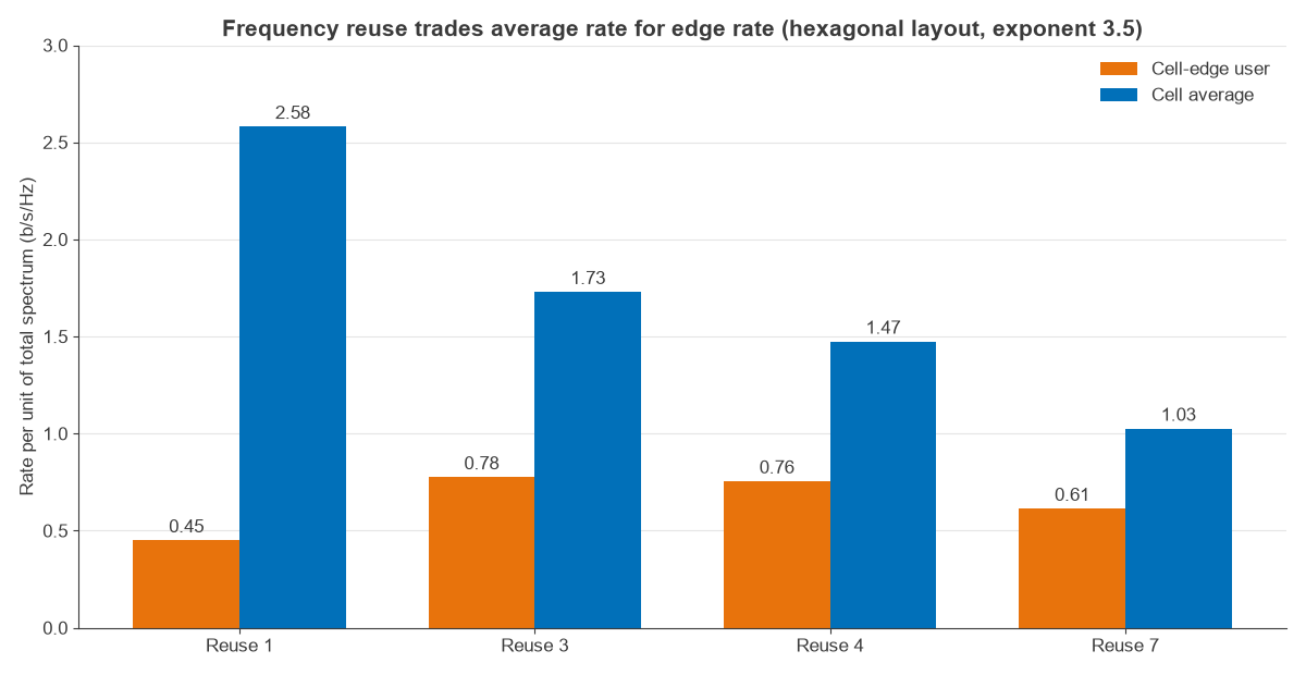
The table comes from a full-load hexagonal grid with path-loss exponent 3.5, summing interferers out to 14 cell radii, and a noise-only SNR of 20 dB at the cell corner, with no shadowing. The cell average leaves out the area within 0.1 R of the site. Rates are shown per unit of total spectrum, after dividing by K.
| Reuse factor K | Nearest co-channel distance | Corner SINR | Corner rate | Cell average rate |
|---|---|---|---|---|
| 1 | 1.73 R | −4.4 dB | 0.45 | 2.58 |
| 3 | 3.00 R | 6.0 dB | 0.78 | 1.73 |
| 4 | 3.46 R | 8.5 dB | 0.76 | 1.47 |
| 7 | 4.58 R | 12.7 dB | 0.61 | 1.03 |
Figure 1 shows the same trade. Moving from reuse 1 to reuse 3 raises the cell-corner rate by 72%, even after spectrum division, and cuts the cell average by 33%. Beyond reuse 3 both measures fall. This is why modern systems use reuse 1 across most of the cell and apply partial protection at the edges, through soft or fractional frequency reuse.
Interference avoidance in space: transmit nulling
With more than one antenna, the transmitter can avoid a victim while using the same frequency at the same time. It picks weights w such that the signal cancels in the victim’s direction:
hvT w = 0
For a single-antenna victim, this takes one of the N spatial dimensions. The serving user keeps N − 1 dimensions, so its mean beamforming gain falls from N to N − 1. For 4 antennas, that is a 1.25 dB loss, from a gain of 4 to a gain of 3.
Nulling depends on knowing the victim’s channel. With a CSI error of normalised mean square error ε, the leakage toward the victim does not vanish, and its mean power equals ε times the unprotected level. Figure 2 confirms this with a 4-antenna simulation over 300,000 channels.
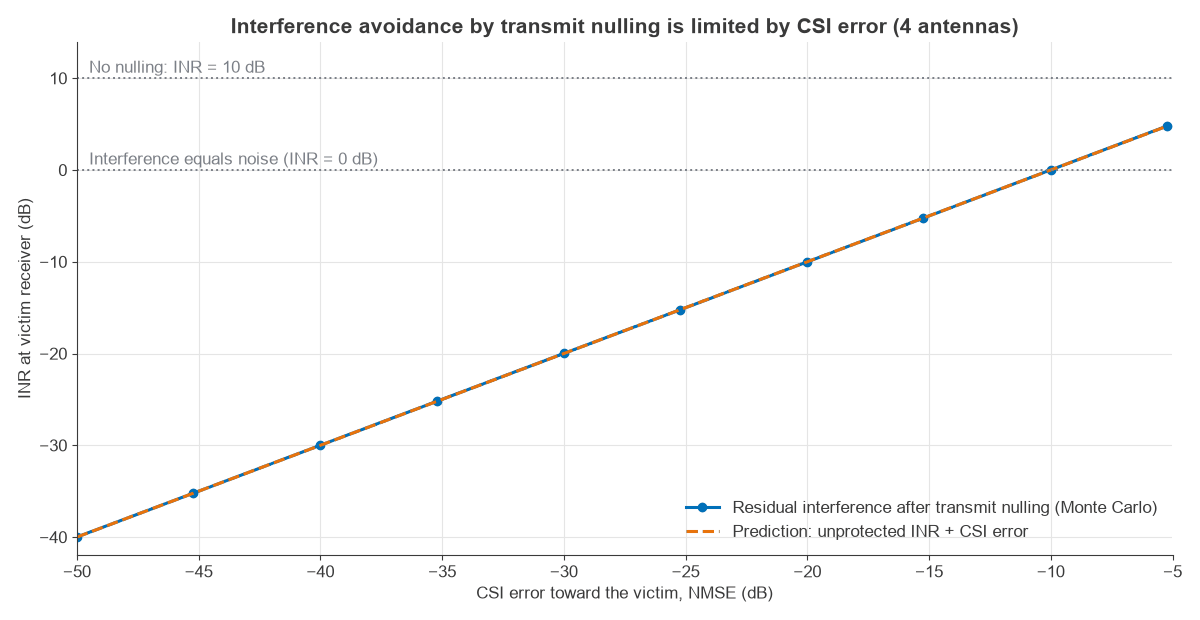
Each 10 dB of better CSI gives 10 dB less leakage. In a reciprocal time-division system, CSI error is often set by calibration and channel ageing, and in a frequency-division system it is set by feedback resolution.
Worked example: is nulling worthwhile?
Base station A has 4 antennas and serves one Rayleigh-fading user at 20 dB SNR per antenna. It also places 10 dB INR at a neighbouring single-antenna victim, whose own link has a steady 20 dB SNR. With CSI error of −20 dB:
| Quantity | Without nulling | With nulling |
|---|---|---|
| Interference at victim (INR) | 10 dB | −10 dB |
| Victim SINR | 9.6 dB | 19.6 dB |
| Victim rate | 3.33 b/s/Hz | 6.52 b/s/Hz |
| Serving-user gain | 4 (6.02 dB) | 3 (4.77 dB) |
| Serving-user mean rate | 8.46 b/s/Hz | 7.98 b/s/Hz |
| Sum of both links | 11.79 b/s/Hz | 14.50 b/s/Hz |
The serving user gives up 0.48 b/s/Hz and the victim gains 3.19 b/s/Hz, a net gain of 23%. A little spatial freedom buys a lot when interference is well above noise. If INR had been 0 dB, the same null would cost almost as much and gain far less. Nulling is best targeted at strong victims only. Beamforming explains the array side of null steering, and MIMO precoding extends the method to multi-user designs.
Avoidance by scheduling: user selection in multi-user MIMO
Scheduling is the cheapest form of avoidance in multi-user MIMO, since it just chooses which users share a resource. Interference between two users depends on how closely their channels align, measured by the correlation ρ between channel vectors. Under zero forcing, separating a pair costs each user a power factor of 1 − |ρ|2:
| Channel correlation magnitude | ZF power penalty |
|---|---|
| 0.3 | −0.41 dB |
| 0.5 | −1.25 dB |
| 0.7 | −2.92 dB |
| 0.9 | −7.21 dB |
Choosing near-orthogonal users avoids most of this. Figure 3 uses a 4-antenna base station and single-antenna Rayleigh users at 20 dB SNR, with a greedy selection of 4 users that picks at each step the user with the most channel energy orthogonal to those already chosen.
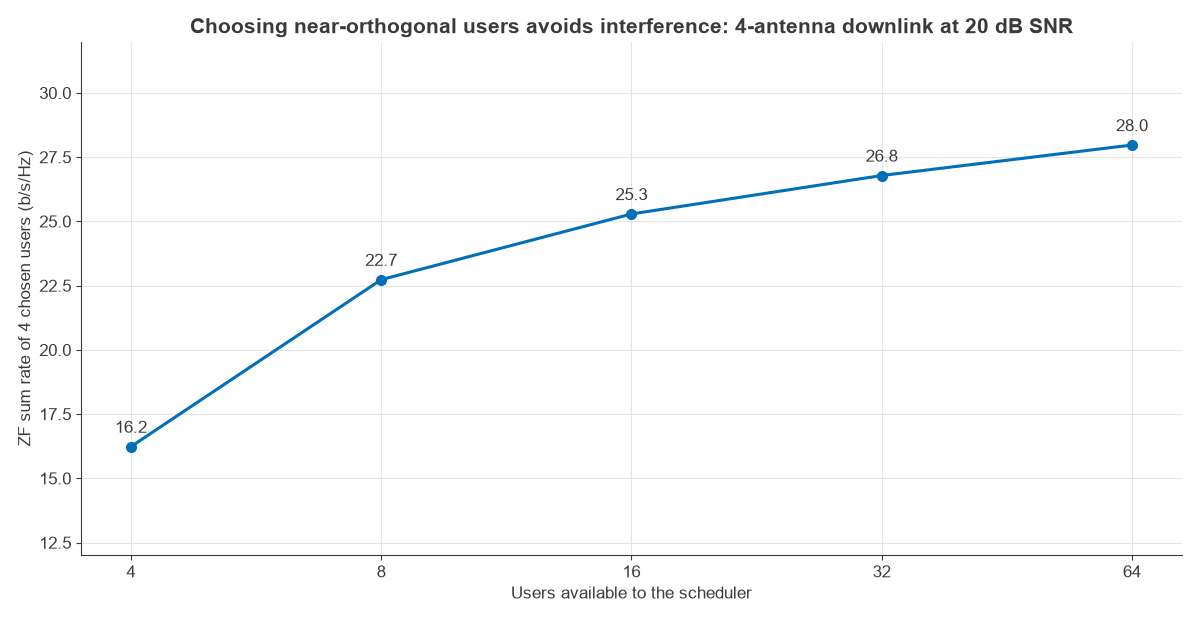
The sum rate rises from 16.2 b/s/Hz with no choice to 22.7 with 8 candidates and 28.0 with 64, a 72% gain with no added power, antennas or bandwidth. Much of it comes with the first doubling of the pool. The result also includes multi-user diversity, since the selected users have strong channels as well as orthogonal ones. The cost is CSI for all candidates and possible unfairness, so practical schedulers balance rate against waiting time.
Iterative algorithms for interference avoidance
When several nodes share a band, each transmitter’s best choice depends on the others. Iterative algorithms approach this by alternating updates. In leakage minimisation, each transmitter selects a beam that minimises the interference it causes, and each receiver then updates its filter, with the sequence repeating until it converges. Signal-to-leakage-and-noise ratio (SLNR) methods handle the conflict between wanted signal and leakage in closed form for each transmitter, which avoids the coupled SINR expressions of the full problem.
Such algorithms usually converge to a local optimum and need CSI to be exchanged or measured over the air. In time-division systems, the reciprocal channel lets nodes learn by listening, which cuts signalling. Convergence time must stay short relative to the channel coherence time, or the solution is stale before it is used.
Interference avoidance technology outside MIMO precoding
Several long-established methods avoid interference with little or no channel knowledge, and they complement MIMO techniques.
- Listen before talk: a Wi-Fi radio senses the channel and defers if it is busy, with energy-detect thresholds typically near −62 dBm and preamble detection near −82 dBm in a 20 MHz channel.
- Adaptive frequency hopping: classic Bluetooth hops across up to 79 channels of 1 MHz and marks bad channels so that it skips them.
- Dynamic frequency selection: 5 GHz devices that detect radar in shared channels move away from it.
- Power control: lowering power to what the link needs reduces interference for everyone. Mean interference falls 1 dB for each 1 dB saved.
- Polarisation: orthogonal polarisations typically give around 10 to 25 dB of isolation in practice, depending on the antennas and environment.
- Sectorisation and tilt: limiting the antenna pattern is spatial avoidance in fixed form. Antenna pattern and downtilt shape how much reaches neighbouring cells.
Physical planning sits beneath all of these. Link geometry from a link budget shows how much margin a design has before any technique is applied. Each of these choices changes the interference environment that the receiver later sees, so they should be set together with antenna and propagation decisions.
Choosing an interference mitigation approach
Start with the cheapest step that addresses the actual cause. Measure first, since a noise rise of several dB can come from a co-channel cell, an adjacent-channel leak or a local fault, and each has a different fix.
- If one neighbour dominates and CSI is available, use transmit nulling or coordinated beams.
- If many weak interferers add up, use power control and fractional reuse.
- If users are correlated, change the user grouping before adding hardware.
- If the source is external and cannot be coordinated, use avoidance in frequency or suppression at the receiver.
- If interference still arrives, move on to cancellation.
Frequently asked questions
What is interference mitigation?
It is any technique that reduces the effect of unwanted signals on a wireless link. It includes avoidance before transmission, suppression during reception and cancellation afterwards. Good designs combine several of them.
What is the difference between interference avoidance and interference cancellation?
Avoidance prevents interference from reaching the receiver, by separating signals in time, frequency, space or power. Cancellation removes it after arrival by reconstructing and subtracting it. Avoidance costs resources at the transmitter, and cancellation costs accuracy and processing at the receiver.
Does interference avoidance need channel state information?
Not always. Frequency reuse, sectorisation, listen before talk and frequency hopping need little or no CSI. Transmit nulling, coordinated beamforming and user selection do need it, and the CSI quality sets how much they achieve.
How deep can a transmit null be?
In a model with only CSI error, the mean residual is ε times the unprotected level, so −20 dB NMSE gives about 20 dB of protection. Calibration errors, phase noise and transmitter EVM set further limits in real hardware.
Related topics
Related reading includes MIMO interference management, interference cancellation, beamforming and MIMO precoding. For CSI, see channel state information. System context is in MIMO, beamforming and phased-array architectures and radio architectures.