


Deep learning-based CSI feedback compresses the channel estimate at the user with a trained encoder network and rebuilds it at the base station with a matching decoder. The aim is to return more accurate channel state information in fewer uplink bits than a fixed codebook, which improves precoding on FDD MIMO links. It works by learning the channels of a given environment, so its main weakness is performance outside that environment.
The channel state information page explains why CSI feedback is needed, and CSI quantization covers conventional reduction methods. This page asks a narrower question: how far can a learned model cut the report, compared with simpler methods, and what does it cost? A small simulation gives numbers throughout.
Why CSI feedback limits MIMO performance
In FDD, uplink and downlink use different frequencies, so the base station cannot measure its downlink channel directly. The user measures it and reports back. The report grows with antennas and bandwidth.
Take 16 base station antennas and 256 subcarriers, with one receive antenna. Converting to the angle-delay domain and keeping the first 16 delay taps leaves 16 × 16 = 256 complex values, or 512 real numbers, which held about 98% of the energy in the channels used below. At 8 bits each, that is 4,096 bits per report. Sending one every 10 ms takes 410 kb/s per user. Multiply by users and receive antennas, and this competes with the uplink data it is meant to help.
NR handles this with codebooks. Type I reports a beam index, which is cheap but coarse. Type II reports several beams with amplitude and phase weights, and costs more. Learned compression tries to do better for the same number of bits.
How deep learning CSI feedback works
The usual design is a two-sided autoencoder.
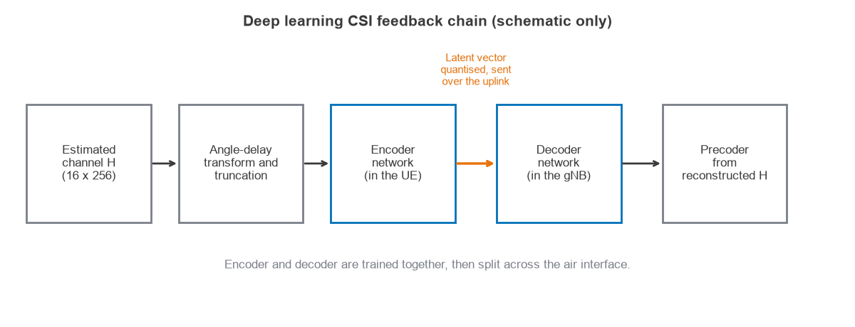
- The user estimates H and transforms it to the angle-delay domain, where the channel is sparse.
- An encoder network maps the matrix to a short latent vector.
- The vector is quantised and sent on the uplink.
- A decoder network at the base station reconstructs the channel.
- The base station derives its precoder from the result.
Training minimises normalised mean squared error (NMSE) over a large set of channels:
NMSE = E[ ||H – Ĥ||2 / ||H||2 ]
CsiNet, published in 2018, made this approach well known by adapting image compression networks to CSI. Later designs add attention layers, or exploit correlation between reports over time. All of them depend on one thing: real channels are not random matrices. Angles and delays follow the site’s geometry, and a model can learn that structure.
Simulation: what compression can achieve
This example tests the idea on a synthetic channel. It models one site: 16 antennas, 20 MHz, one user-dependent cluster at a random angle within ±60 degrees, and two reflector clusters at fixed angles. There are 9,000 training channels and 1,000 test channels.
Sparsity alone goes a long way. In the angle-delay domain, 19 of the 256 coefficients hold 90% of the energy on average, and 90 hold 99%. Three methods were compared, with latent values taken at 6 bits each:
- Largest coefficients. Send the strongest values with 8-bit position indices and 6 bits each for real and imaginary parts, or 20 bits per coefficient. This needs no training.
- PCA. A linear encoder trained on the site.
- Autoencoder. A fully connected network with one 256-unit hidden layer on each side, trained on the site.
| Bits per report | Latent values | PCA NMSE (dB) | Autoencoder NMSE (dB) | Autoencoder at a new site (dB) |
|---|---|---|---|---|
| 768 | 128 | -17.2 | -17.1 | -3.4 |
| 384 | 64 | -8.2 | -8.2 | -1.7 |
| 192 | 32 | -4.7 | -4.7 | -0.6 |
| 96 | 16 | -3.4 | -3.4 | -0.1 |
The largest-coefficient method gave -16.5 dB at 1,280 bits, -12.3 dB at 640 bits, -9.5 dB at 320 bits and -7.1 dB at 160 bits. The NMSE values above use unquantised latent vectors, so the bit counts assume 6-bit quantisation adds little further error. They are also measured against the 16-tap channel, so the energy dropped by truncation is not counted.
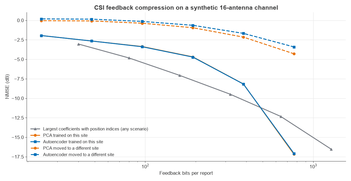
Three results stand out.
First, at about -17 dB the trained methods need 768 bits, against 1,280 bits for the coefficient method, which is 40% fewer. That is an 81% cut from the raw 4,096-bit report.
Second, the small autoencoder did no better than PCA. With this simple network and data set, it learned something close to a linear projection. The non-linear gains reported for deep convolutional networks need larger models and far more training data than this example, so these figures are a baseline and not a limit.
Third, at low bit counts, the coefficient method beat the trained models. Below about 500 bits it had lower error at the same size, because the random user cluster has too much variation for a small linear code.
Why NMSE translates into beamforming gain
NMSE is an indirect measure. What matters is how well the beam built from Ĥ points at the true channel. A useful measure is the squared correlation between h and ĥ on each subcarrier, and the gain falls by that factor. In this simulation:
| Case | Squared correlation | Beamforming loss (dB) |
|---|---|---|
| Autoencoder, 768 bits, same site | 0.982 | 0.08 |
| Autoencoder, 384 bits, same site | 0.880 | 0.56 |
| Autoencoder, 192 bits, same site | 0.711 | 1.48 |
| Autoencoder, 768 bits, new site | 0.593 | 2.27 |
For single-user beamforming, even 192 bits loses only 1.5 dB. Channel estimation errors shows why this is not the full story: MU-MIMO depends on accurate nulls, and it needs much lower error than single-user links.
The generalisation problem
Moving the trained autoencoder to a different site, with six clusters and wider angular spread, took the NMSE at 768 bits from -17.1 dB to -3.4 dB. The learned code was built for the first site’s geometry, and on the new site the reconstruction is too poor for multi-user precoding and costs 2.3 dB even on a single-user beam. The coefficient method, which assumes nothing about the site, does not have this weakness.
Published work reaches similar conclusions, and the remedies are all practical trade-offs:
- Train on many mixed environments, accepting less compression per site.
- Fine-tune online with data collected at the site, which needs a data path and storage.
- Keep several models and switch between them, with a selection procedure.
- Monitor performance and fall back to a codebook when the model drifts.
Practical costs of deep learning CSI feedback
- Model size at the user. The 192-bit autoencoder’s encoder holds about 140,000 parameters, against about 16,000 for PCA. Published deep models are often larger. That cost falls on the handset, with its battery and memory limits.
- Two-sided compatibility. The encoder and decoder must match. In a real network they come from different vendors, so the handset and network sides need agreed training or an agreed interface.
- Standardisation. 3GPP has studied AI and machine learning for CSI feedback, and two-sided model coordination is one of the harder questions.
- Testing. Conformance is hard to define for a model that changes per site. A fixed codebook has a known, repeatable result.
- TDD. Reciprocity avoids most of this problem, so the benefit is mainly in FDD and in partial-reciprocity cases.
The result for engineers is a clear ordering. Exploit sparsity first, because the angle-delay transform provides most of the gain at no training cost. Then add learning where the channels are stable enough to learn and the feedback saving justifies the extra system complexity.
Frequently asked questions
What is CSI feedback in MIMO systems?
It is the report a receiver sends so that the transmitter knows the channel. FDD links rely on it because the downlink channel cannot be measured directly at the base station.
How does deep learning reduce CSI feedback overhead?
An encoder trained on real or simulated channels maps the matrix to a short vector, and a decoder rebuilds it. Because channels have structure, the short vector can hold most of the information.
Is deep learning better than a codebook for CSI feedback?
It can be, on channels like those it was trained on. In this simulation a trained model cut the raw report by 81% at -17 dB NMSE, but lost most of that performance at a new site. A codebook behaves the same everywhere.
Does 5G use deep learning for CSI feedback?
Deployed NR links use Type I and Type II codebooks. AI-based CSI feedback has been studied in 3GPP, so it remains an area of standards work and not a general deployed feature.
Related topics
Massive MIMO spectral efficiency shows why feedback becomes harder as arrays grow, and beamforming techniques in cellular systems covers codebook and reciprocity methods. User scheduling in MIMO systems shows how CSI quality limits multiuser gain.