

Frequency domain analysis describes an RF signal by how much power it has at each frequency, not by how its voltage changes over time. In RF design it is the main way to measure harmonics, intermodulation, noise, spurs and occupied bandwidth, using a spectrum analyzer or a fast Fourier transform (FFT). The results depend on resolution, window and noise settings, so those need to be understood as well.
Time-domain views show amplitude and timing, but faults such as a spur 70 dB below the carrier cannot be seen on an oscilloscope. This article covers the mathematics briefly, then the practical FFT choices, then the standard RF measurements.
Why Frequency Domain Analysis Matters in RF Design
Linear RF circuits are defined by their frequency response. A filter, a matching network or an amplifier treats each frequency separately, with its own gain and phase, so analysis at each frequency is simpler than solving differential equations. Nonlinear behaviour also shows up clearly, since it produces new frequencies that were not present at the input. Most RF specifications, from ACLR and ACPR to spurious emissions, are written in the frequency domain.
From the Time Domain to the Frequency Domain
The Fourier transform converts a waveform x(t) to a spectrum X(f):
X(f) = ∫ x(t) exp(−j2πft) dt
For a periodic signal, the spectrum is a set of lines at the fundamental and its harmonics. For instance, an amplifier driven into saturation turns a sine wave into something close to a square wave. Figure 1 shows the output of a tanh limiter driven by a 100 MHz sine, with odd harmonics at −13.7, −24.4, −34.8 and −45.1 dBc. The even harmonics vanish, because the transfer curve is symmetric.
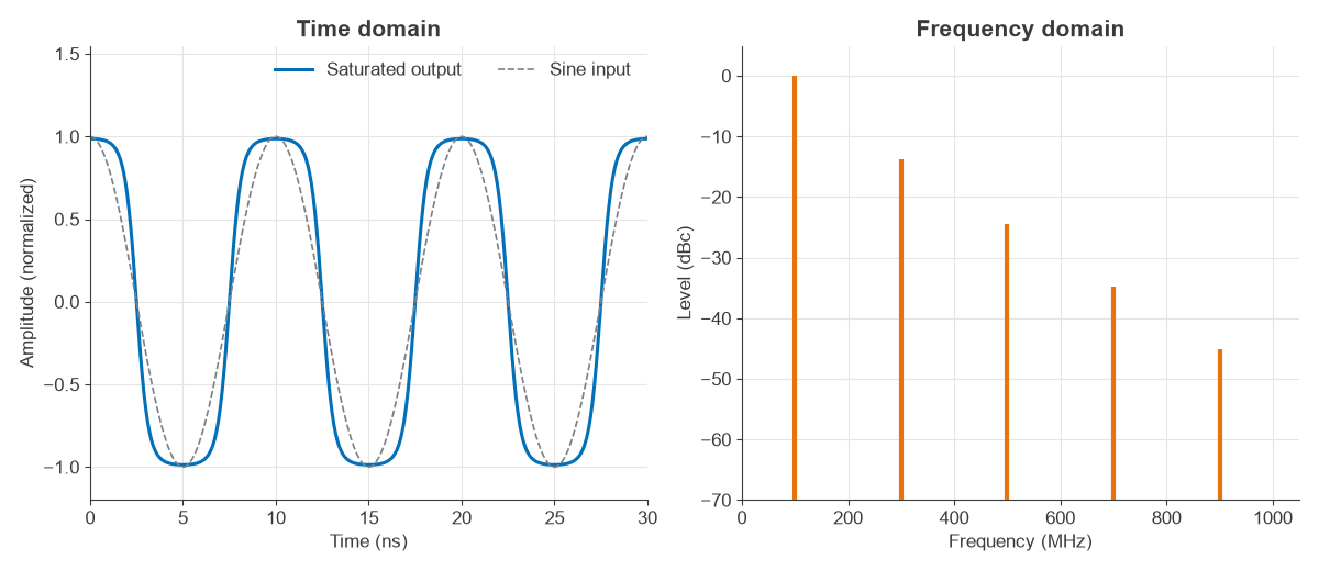
Energy is conserved between the two views, which is Parseval’s theorem. The mean squared value computed for this waveform is 0.7230 in both domains.
The DFT and FFT in Signal Processing
Measured data is sampled, so the working tool is the discrete Fourier transform (DFT), and the FFT is a fast algorithm for it. For N samples at rate fs:
- Bin spacing: Δf = fs/N, which is also 1/(record time).
- Span: 0 to fs/2 for a real signal, or −fs/2 to +fs/2 for complex I/Q.
- Processing gain: 10 log(N/2) for a tone against white noise.
Resolution depends on record length only. Adding zeros interpolates the plot, yet it does not separate two close tones. Anything above fs/2 aliases, so an anti-alias filter must precede the ADC.
Worked Example: FFT Settings for an ADC Capture
A 12-bit ADC samples at 100 MS/s and the FFT uses 4096 points.
- Bin spacing: 100 MHz / 4096 = 24.41 kHz, with a 40.96 µs record.
- Ideal ADC SNR: 6.02 × 12 + 1.76 = 74.0 dB over 0 to 50 MHz.
- Processing gain: 10 log(4096/2) = 33.1 dB.
- Noise floor per bin: −74.0 − 33.1 = −107.1 dB relative to a full-scale sine.
- With a Hann window, noise bandwidth rises to 1.5 bins, or 36.6 kHz, lifting the floor 1.76 dB to −105.3 dB.
A simulation of a quantized sine averaged over 200 records measured −107.1 dB with a rectangular window, which matches. Note that the displayed floor is well below the ADC’s 74 dB SNR figure. A spur at −90 dB is easily visible in this plot, and doubling N lowers the floor by another 3 dB.
Spectral Leakage and Window Functions
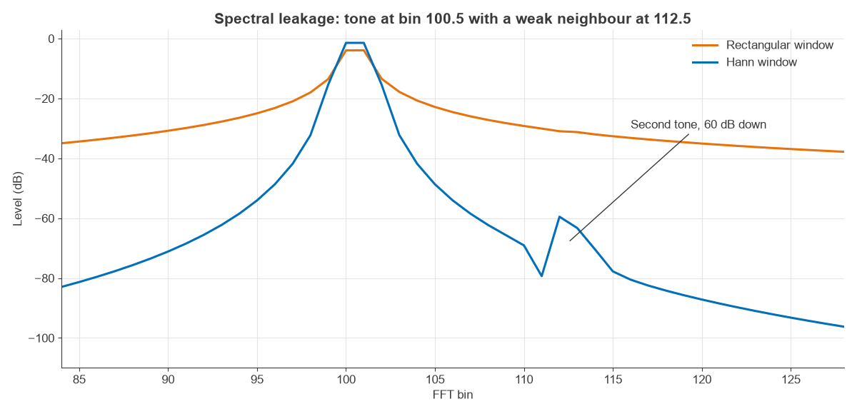
An FFT treats the record as if it repeats forever. If a tone does not fit a whole number of cycles, the join creates a discontinuity, and power spreads across all bins. This is spectral leakage. Multiplying the data by a window that tapers to zero reduces leakage, at the cost of wider peaks.
| Window | Noise bandwidth (bins) | Worst-case scallop loss | First sidelobe |
|---|---|---|---|
| Rectangular | 1.00 | 3.92 dB | −13 dB |
| Hann | 1.50 | 1.42 dB | −31 dB |
Scallop loss is the level error for a tone halfway between two bins. Choose a rectangular window only when the capture is coherent, with an exact integer number of cycles. Choose Hann as a general default, and a flat-top window for amplitude accuracy. For a strong tone in dynamic range tests, a window with lower sidelobes such as Blackman-Harris is appropriate.
Swept Spectrum Analyzers and Resolution Bandwidth
A traditional spectrum analyzer mixes the input down and passes it through a narrow IF filter, the resolution bandwidth (RBW). The displayed noise level follows:
Noise (dBm) = −174 + 10 log(RBW) + NF
With a 24 dB analyzer noise figure, this gives −100 dBm at 100 kHz RBW, −110 dBm at 10 kHz and −120 dBm at 1 kHz. Narrower RBW reveals weaker signals but slows the sweep, roughly as span/RBW². Noise falls 10 dB for each decade of RBW while a CW tone stays the same height, which is a quick way to tell the two apart. Readings must be corrected to dBm/Hz for noise; see thermal noise.
Measuring Harmonics and Intermodulation in the Frequency Domain
Harmonics are the simplest test. They are usually removed by a low-pass filter, and they appear at integer multiples of the carrier. Intermodulation is harder because the products fall close to the wanted signal, so a filter cannot remove them.
Two-tone test and third-order intercept
Two equal tones f1 and f2 are applied to the device. Third-order products fall at 2f1 − f2 and 2f2 − f1. Each product grows 3 dB per dB of input, so a straight-line extrapolation gives the output third-order intercept:
OIP3 = Ptone + (Ptone − PIM3) / 2
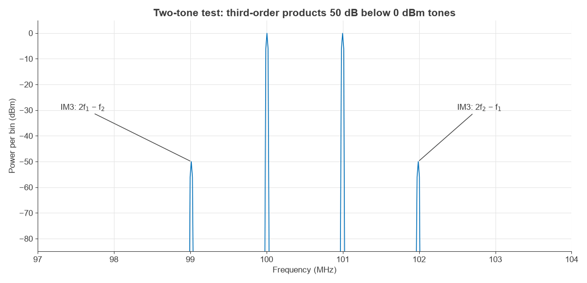
With tones at −0.08 dBm and products at −50.0 dBm in the simulation, OIP3 = −0.08 + 49.92/2 = +24.9 dBm, close to the +25 dBm set in the model. A real measurement needs the analyzer’s own distortion to be well below this, so the input attenuator is raised until the reading stops changing.
Other Frequency Domain Measurements in RF Design
- Occupied bandwidth and channel power integrate noise-like signals over a stated band, so they do not depend on RBW after correction.
- Adjacent channel power measures spectral regrowth from a nonlinear amplifier, which is linked to EVM and PAPR.
- Phase noise measures noise close to a carrier, as dBc/Hz at a given offset.
- S-parameters from a vector network analyzer give complex frequency response, and an inverse FFT of that gives a time-domain reflection plot for finding faults.
Modulated waveforms also have clear spectral signatures, such as the sidebands of AM, the Bessel lines of FM, and the sinc lobes of FSK and ASK. Pulse shaping in PAM is designed entirely in frequency terms.
Choosing Time or Frequency Domain Analysis
Neither view replaces the other. Time domain suits rise time, settling, pulse shape and transient events, and frequency domain suits filters, spurs, distortion and noise. Real-time analyzers and spectrograms combine the two by running overlapping FFTs, so a brief hop or burst can be seen in both.
Frequently asked questions
What is frequency domain analysis?
It represents a signal or a system by its amplitude and phase at each frequency. Engineers obtain it from a Fourier transform, an FFT of sampled data or a spectrum analyzer.
What sets the resolution of an FFT?
The record time. Bin spacing is fs/N, or one over the capture length, and the window then widens each peak by a further factor. Zero padding does not add true resolution.
What is the difference between RBW and FFT bin width?
RBW is the width of a swept analyzer’s IF filter. In an FFT, bin width multiplied by the window’s noise bandwidth is the equivalent number, so 1.5 bins for Hann.
Why does a spectrum analyzer noise floor change with RBW?
Noise power collected is proportional to bandwidth, so the displayed noise changes 10 dB for each decade of RBW. A narrowband tone remains the same height.
Related topics
Frequency planning is described in importance of frequency in RF communication, and modulated spectra in amplitude modulation and demodulation and continuous wave modulation. The RF design and RF noise hubs cover measurements and link budgets.