


Amplitude and power control techniques in RF design hold a signal at the right level despite changes in gain, temperature, load and input strength. Transmitters use automatic level control, which compares a detected output with a setpoint and adjusts an attenuator or the amplifier. Receivers use automatic gain control, which keeps the signal inside the range of the mixer and ADC.
Both are feedback loops built from the same parts: a variable gain element, a detector, a reference and a loop filter. This article covers how those loops work, how to size them, and how the choice affects efficiency. The measurement side is covered in measuring amplitude and power in RF signals, and the units in understanding power in RF systems.
Why RF amplitude control is needed
A transmitter needs accurate output power. Too little reduces range, and too much breaks regulatory limits, drives the amplifier into compression and raises adjacent channel power. Yet transistor gain can move by decibels across temperature, supply and frequency.
A receiver has the opposite problem. Its input can vary by 80 dB or more between a distant signal and a nearby one. No fixed gain can keep both within the range of an ADC, so strong signals clip while weak ones disappear into quantization noise.
Open-loop and closed-loop power control
Open-loop control sets a gain from a calibration table, indexed by frequency, temperature and requested power. It is fast and needs no detector, but it can correct only what was calibrated. Closed-loop control measures the output and corrects the error, so it also handles drift nobody modelled. Its accuracy then depends on the detector and coupler, and it takes time to settle. Practical radios often combine both, with a table for coarse setting and a loop or periodic detector reading for trim.
Automatic level control in a transmitter
Figure 1 shows a typical automatic level control (ALC) loop. A directional coupler samples the output, an RF power detector converts it to a voltage, and an integrator compares that with a setpoint from a DAC. The error drives a variable attenuator ahead of the amplifier.
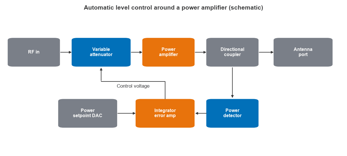
The control element comes before the amplifier because an attenuator after it would waste output power. Detector choice follows the waveform. A diode envelope detector is simple and fast, a logarithmic detector gives a wide dB-linear range, and an rms detector reads true power regardless of crest factor, which matters for OFDM.
Worked example: holding +30 dBm
Take a transmitter with a +30 dBm target and forward gain that can drift by ±2 dB.
- Detector drive: a 20 dB coupler and a 10 dB pad put the detector at 30 − 20 − 10 = 0 dBm, in the middle of a typical range.
- Loop correction: a proportional loop with loop gain 20 reduces the error to ±2 / (1 + 20) = ±0.095 dB. An integrator takes the steady-state error toward zero.
- Coupler error: with an antenna return loss of 10 dB and 20 dB coupler directivity, reflected power reaches the detector 30 dB below the forward sample. In the worst phase it adds 20 log10(1 + 10−30/20) = 0.27 dB of voltage error.
- Settling: a first-order loop with a time constant of 20 µs has a bandwidth of 8.0 kHz, and settles to within 1% of a step in 4.6 time constants, or 92 µs.
The example shows the central rule of closed-loop control: the loop removes forward-path drift, but it inherits every error in the sensing path. Detector temperature drift and coupler directivity set the final accuracy, so they deserve the design margin. The loop also must not track the signal’s own envelope. If it is faster than the modulation, it will flatten the wanted amplitude, so bandwidth must stay below the lowest significant envelope frequency, or the detector must average over it.
Power control in RF amplifiers
Output power can be reduced at the input or at the supply. Input control is simple, but a fixed supply wastes power at back-off. For an ideal class B stage, efficiency is 78.5% at saturation and falls as the square root of output power. At 6 dB back-off it is 39.4%, at 10 dB 24.8% and at 20 dB 7.9%, as plotted in Figure 2.
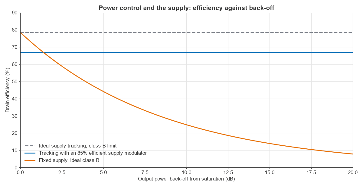
Reducing the supply along with the power avoids this. Average power tracking changes the supply slowly according to the average power level. Envelope tracking follows the instantaneous envelope, and needs a fast supply modulator. With an ideal stage and an 85% efficient modulator, the combined efficiency is about 66.8% across the range, ignoring device limits at low voltage. Real gains are much smaller at deep back-off, and the amplifier’s gain and phase now vary with supply, so PA linearization and the class of operation, described in power amplifier classes, must be designed together with it.
Network-side power control adds another layer in cellular systems. The base station commands each handset up or down in small steps, using closed-loop commands on top of an open-loop path loss estimate. This saves battery and limits interference, and it is the system-level reason the RF chain needs a wide, accurate control range.
Automatic gain control in a receiver
An automatic gain control (AGC) loop measures the signal level, usually after filtering or in the digital baseband, and adjusts gain to keep the ADC input near a target. Filtering first matters, since a detector placed ahead of channel selection also responds to adjacent signals.
Worked example: sizing the AGC range
Consider a receiver with an input range of −100 to −20 dBm and an ADC with 0 dBm full scale. The target is −12 dBFS, which leaves headroom for a crest factor near 12 dB.
- Gain needed: −12 − (−100) = 88 dB at the weakest signal, and −12 − (−20) = 8 dB at the strongest.
- Range: 88 − 8 = 80 dB of total gain control.
- Split: with a fixed 30 dB front end, the remaining stages must span +58 to −22 dB.
- Resolution: 0.5 dB steps over 80 dB give 160 states, which an 8-bit control word covers.
Gain distribution across the receive chain
Where the gain is removed matters as much as how much. At low signal levels, all gain stays in place, with the highest gain in front to protect cascaded noise figure. As the signal grows, later stages are reduced first, so noise figure holds steady. Near the top of the range, the LNA is stepped down or bypassed to protect linearity and intercept point. The input signal is then strong enough that the higher noise figure has little effect. Each change of gain should occur where there is SNR to spare, and the switching points need hysteresis so the receiver does not chatter between states. How the stages are arranged depends on the choices in receiver architecture comparison.
AGC dynamics: dB-linear control
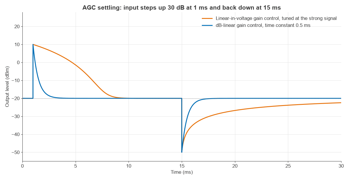
A loop’s speed depends on its loop gain, and in a gain-control loop that can depend on the signal level. A dB-linear variable gain amplifier has a constant slope in dB per volt. With a logarithmic detector, the loop becomes linear in decibels, so settling time does not depend on level. That is the reason for pairing the two.
Figure 3 compares this with a gain element that is linear in voltage, tuned for the strong-signal case. For a 30 dB step, the dB-linear loop with a 0.5 ms time constant settles to within 1 dB in 1.7 ms, in both directions. The linear element takes 7.5 ms to clear an overload, and is still 2.4 dB short of target 15 ms after the signal falls, since its dB slope depends on gain.
Attack and decay are usually set separately. Fast attack limits clipping, while slower decay avoids pumping during brief fades or between packets. Burst systems instead measure on a preamble and freeze the gain for the packet. Steps in gain also disturb the phase of the signal, so an OFDM receiver should not change gain in the middle of a symbol.
Choosing an amplitude control method
| Need | Usual method |
|---|---|
| Accurate transmit power over temperature | Closed-loop ALC with an rms or log detector |
| Very fast power steps | Open-loop table with periodic detector trim |
| Efficiency at back-off | Average power tracking or envelope tracking |
| Wide receive range | Stepped LNA plus VGA or digital AGC |
| Burst reception | Preamble measurement and frozen gain |
Frequently asked questions
What is the difference between AGC and ALC?
AGC usually refers to a receiver loop that keeps a varying input at a constant output level. ALC usually refers to a transmitter loop that holds the output power at a setpoint despite changes in gain.
Why does the attenuator go before the power amplifier?
Attenuation after the amplifier throws away output power and creates heat. Placed before it, the attenuator handles small signals and controls drive level at little cost.
How fast should a power control loop be?
Faster than the drift or fading it must correct, and slower than the signal’s amplitude modulation. Otherwise it will flatten the envelope and distort the signal.
Why use a dB-linear variable gain amplifier in AGC?
It keeps the loop’s dynamics independent of signal level when paired with a log detector, so settling time is the same across the range.
Related topics
These loops are part of the RF design area, with related stages in the RF amplifiers hub. The RF calculators help with level planning.