


Diversity in antenna systems means receiving or sending a signal through two or more antennas that fade independently, and it is one of four diversity techniques in wireless communication. The others separate the copies in polarisation, frequency or time. Each technique works only if the copies are far enough apart to decorrelate, so the useful design question is how far apart is far enough.
This article answers that question for each dimension, with formulas and numbers for spacing, hop distance and interleaver depth. The mechanics of combining the branches and the fade margin they save are covered in transmit and receive diversity.
Diversity techniques in wireless communication at a glance
Every diversity technique relies on the same statistics. A multipath channel fades deeply only occasionally, so two independent copies rarely fade together. The measure of independence is the envelope correlation between branches, and values below about 0.5 to 0.7 are usually treated as good enough. Each dimension has its own quantity that sets that correlation.
| Technique | What decorrelates the copies | Rule of thumb | Main cost |
|---|---|---|---|
| Space diversity | Antenna separation d | About 0.4λ with scatter all around, many λ at an elevated site | Extra antennas and chains |
| Polarisation diversity | Orthogonal polarisations | Co-located, needs depolarising multipath | Dual-feed antenna, possible branch imbalance |
| Frequency diversity | Frequency separation Δf | Δf above coherence bandwidth, Bc ≈ 1/(5στ) | Extra bandwidth |
| Time diversity | Time separation Δt | Δt above coherence time, Tc ≈ 0.423/fd | Latency |
Diversity in antenna systems: space and polarisation
Space diversity, also called spatial diversity, is what most engineers mean by antenna diversity. Two antennas see different sums of the same multipath waves, and the required spacing depends on the spread of angles the waves arrive from.
Spatial diversity at a handset
With scatter arriving equally from all directions (the Clarke model), the envelope correlation between two vertical antennas spaced d apart is:
ρe ≈ J02(2πd/λ)
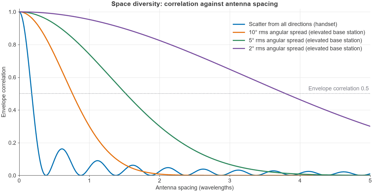
The first null is at d = 0.383λ, which is 12.8 cm at 900 MHz, 4.8 cm at 2.4 GHz and 3.3 cm at 3.5 GHz. Correlation falls quickly before that point: it is 0.82 at 0.1λ and 0.41 at 0.2λ, so even a small device gets useful decorrelation. Figure 1 shows the curve in blue.
Spatial diversity at an elevated base station
An antenna above the clutter sees scatterers only near the user, so waves arrive from a narrow range of angles. For a Gaussian angular spread of σθ radians around broadside, a small-angle result is:
ρe ≈ exp[-(2πd σθ/λ)2]
Setting ρe = 0.5 gives the spacings in the table. A Monte Carlo average over a 5° Gaussian spread agreed with this formula at d = 1λ, giving 0.74. This is why tower sites space their receive antennas by many wavelengths, while a phone manages with a few centimetres.
| Rms angular spread | Spacing for ρe = 0.5 | At 900 MHz | At 3.5 GHz |
|---|---|---|---|
| 10° | 0.76λ | 0.25 m | 6.5 cm |
| 5° | 1.52λ | 0.51 m | 13 cm |
| 2° | 3.80λ | 1.26 m | 33 cm |
Polarisation diversity and pattern diversity
Polarisation diversity uses two orthogonal polarisations, often ±45° slant, in one radome. Reflections and scattering rotate the polarisation differently from path to path, so the two ports fade largely independently with no physical spacing. The catch is level: if the channel keeps most power in one polarisation, the second branch is weaker, and the diversity gain shrinks with that imbalance. Pattern diversity is a related method, where antennas at the same point look in different directions. Patterns that overlap little also pick up different multipath waves. See antenna parameters for how polarisation and pattern are defined.
Frequency diversity in wireless communication
Frequency diversity sends information on carriers separated by more than the coherence bandwidth, so that a multipath notch hits only part of it. For a channel with an exponential power delay profile and rms delay spread στ, the envelope correlation between two frequencies is:
ρe(Δf) = 1 / [1 + (2πΔf στ)2]
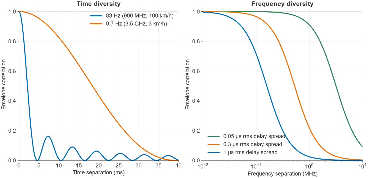
The common rule Bc ≈ 1/(5στ) corresponds to a correlation of 0.39 on this model. Definitions of coherence bandwidth vary, so treat it as an estimate. A delay spread of 1 µs gives 200 kHz, 0.3 µs gives 667 kHz and 50 ns gives 4 MHz.
A wideband signal gets frequency diversity on its own account. A 20 MHz channel with 0.3 µs delay spread contains about 30 coherence bandwidths, and OFDM exploits them by coding across subcarriers. The same channel with 50 ns delay spread contains only about 5, so it benefits far less. Frequency hopping does the same job one hop at a time, and a RAKE receiver in a spread spectrum system collects the resolved paths, which works when the chip period is shorter than the delay spread. The effect of these fades on subcarriers is covered in wireless channel fading and OFDM.
Time diversity in wireless communication
Time diversity repeats or spreads coded data over intervals longer than the coherence time. Interleaving, coding and automatic retransmission all use it. The maximum Doppler shift is fd = v f/c, and for Clarke scattering the correlation at time separation Δt is:
ρe(Δt) = J02(2πfdΔt)
A widely used estimate of coherence time is Tc ≈ 0.423/fd. The key limit is that time diversity needs movement. A stationary user has almost no Doppler spread, so an interleaver spreads the data over a channel that has not changed. It also costs latency, because the receiver must wait for all of the interleaved block. Figure 2 plots both the time and frequency correlation curves.
Worked example: sizing diversity for a link
Take three checks for a cellular link: the time diversity available from a 10 ms interleaver, the bandwidth needed for frequency diversity, and the spacing for space diversity. The table covers the time check at two carriers and two speeds.
| Carrier and speed | Doppler fd | Coherence time Tc | Independent blocks in 10 ms |
|---|---|---|---|
| 900 MHz, 100 km/h | 83.4 Hz | 5.07 ms | About 2 |
| 900 MHz, 3 km/h | 2.50 Hz | 169 ms | 1 |
| 3.5 GHz, 100 km/h | 324 Hz | 1.30 ms | About 7.7 |
| 3.5 GHz, 3 km/h | 9.73 Hz | 43.5 ms | 1 |
The interleaver gives real diversity only to the fast users. At walking pace it gives none on either carrier, and stretching it to 40 ms still gives 1 block at both, since 40 ms is below Tc.
Now suppose the slow case is a 900 MHz sensor with a 200 kHz signal and 1 µs delay spread. The signal is one coherence bandwidth wide, so it has little frequency diversity of its own. Hopping by more than 200 kHz would provide some, and two antennas spaced 13 cm apart would provide independent branches at once. For a device that does not move and has a narrow channel, space or polarisation diversity, or hopping, are the practical options.
What branch correlation costs
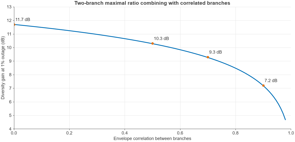
Imperfect separation does not remove the benefit. For two-branch maximal ratio combining in Rayleigh fading, with complex correlation r between branches, the combined SNR behaves like two independent branches with mean powers 1 + |r| and 1 – |r|. Taking ρe ≈ |r|2, the gain at 1% outage is as follows, where a single antenna needs a mean SNR 20.0 dB above threshold:
| Envelope correlation | Mean SNR needed above threshold | Gain over one antenna |
|---|---|---|
| 0 | 8.3 dB | 11.7 dB |
| 0.25 | 8.9 dB | 11.1 dB |
| 0.5 | 9.7 dB | 10.3 dB |
| 0.7 | 10.7 dB | 9.3 dB |
| 0.9 | 12.8 dB | 7.2 dB |
A correlation of 0.7 costs only 2.4 dB of a possible 11.7 dB, which is why the usual threshold is so relaxed. Pushing spacing further yields little once correlation is below about 0.5. The closed-form curve is in Figure 3.
Frequently asked questions
What is diversity in wireless communication?
It is the use of two or more independently fading versions of a signal, so that a deep fade on one does not stop the link. The copies can be separated in space, polarisation, frequency or time. It improves reliability, and it does not by itself raise the peak data rate.
What is diversity in an antenna?
A single antenna does not provide diversity unless it has two ports with different polarisations or patterns. Antenna diversity normally means two or more antennas placed or polarised so that they fade independently. The receiver or transmitter then combines or selects them.
What is the difference between space diversity and frequency diversity?
Space diversity needs extra antennas and no extra spectrum, while frequency diversity needs extra spectrum and no extra antennas. Space diversity depends on angular spread, and frequency diversity depends on delay spread. Many modern links, such as MIMO-OFDM, use both.
How far apart should diversity antennas be?
About 0.4λ is enough with scatter from all directions, which is about 3.4 cm at 3.5 GHz. An elevated antenna with 5° angular spread needs about 1.5λ for a correlation of 0.5, and a narrower spread needs proportionally more.
Related topics
For how the branches are combined, see diversity techniques for SIMO and MISO systems. Transmit diversity covers space diversity without extra receive antennas, and MIMO and multiple antenna systems puts diversity next to array gain and multiplexing. The wider channel background is in antennas and propagation in radio design and the RF fundamentals hub.