

MIMO interference management is the choice of how a multi-antenna system handles signals it does not want: ignore them, suppress them at the receiver, cancel them, avoid them at the transmitter, or turn them into cooperation. No single technique is best, because the right choice depends on how strong the interference is compared with the wanted signal, how much channel knowledge is available and how much the network nodes can coordinate.
This page is the decision guide for those options, with one scenario computed across all of them. Two companion articles go deeper on single branches: interference cancellation in MIMO systems covers removing interference after it arrives, and interference avoidance and mitigation covers preventing it from arriving.
Types of interference in MIMO systems
The word covers several distinct mechanisms, and each is handled in a different place.
| Interference type | Source | Usually handled by |
|---|---|---|
| Inter-stream | Other streams of the same user | Receiver detection or SVD precoding |
| Inter-user | Other users sharing the time and frequency resource | Multi-user precoding |
| Inter-cell | Neighbouring base stations or their users | Coordination, receive suppression |
| Pilot contamination | Reused pilot sequences in nearby cells | Pilot planning, power control |
| Self-interference | A node’s own transmitter in full duplex | Isolation and cancellation |
| External | Other systems in the band | Filtering, avoidance, spatial nulls |
The inter-stream and inter-user cases sit within one transmitter and are controlled by it. The harder cases cross node boundaries, where channel knowledge and timing are not shared by default.
How strong interference changes the best strategy
Intuition says that weak interference is harmless and strong interference is fatal. Information theory says something more interesting. For two symmetric single-antenna links, define the interference level α = log(INR)/log(SNR). The generalised degrees of freedom per user, a high-SNR measure of achievable rate, follow the W curve in Figure 1:
- α ≤ 1/2: 1 − α
- 1/2 ≤ α ≤ 2/3: α
- 2/3 ≤ α ≤ 1: 1 − α/2
- 1 ≤ α ≤ 2: α/2
- α ≥ 2: 1
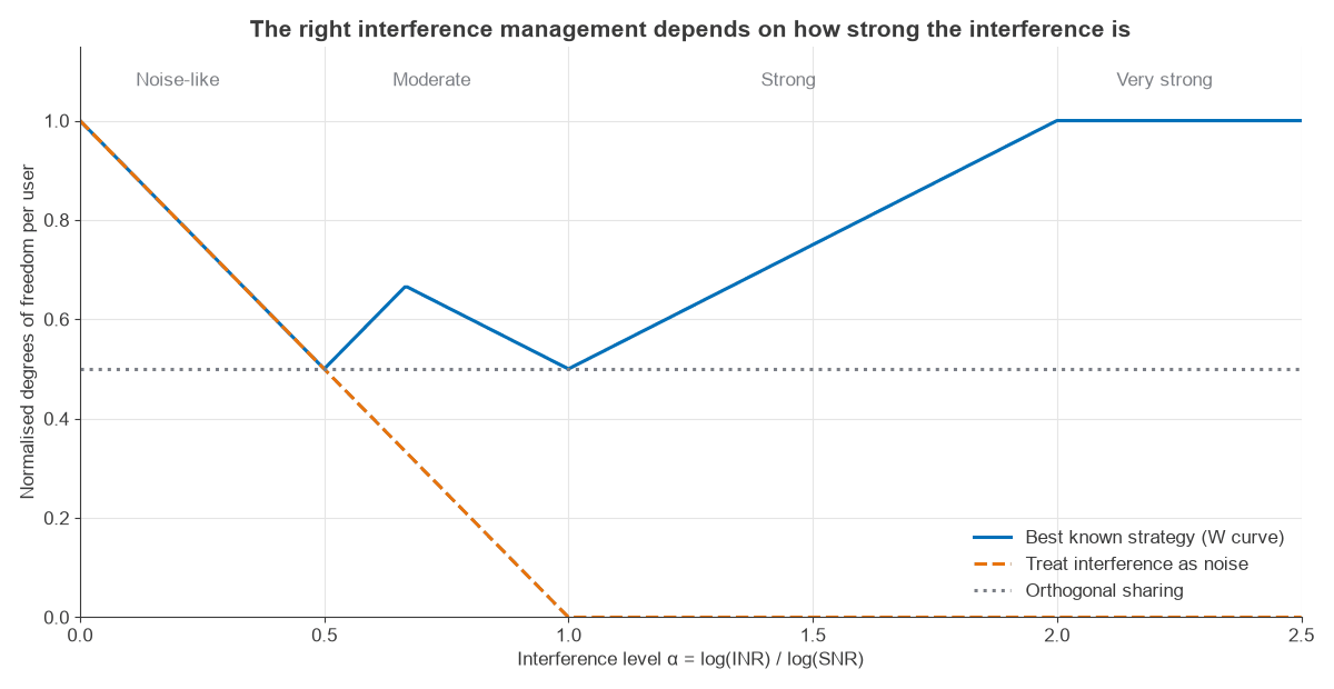
The curve splits into regimes with different engineering answers. Below α = 1/2, treating interference as noise is near-optimal. Around α = 1 the two signals are similar in strength, nothing can be decoded cleanly and orthogonal sharing is close to the best available. At α ≥ 2, interference is so strong that a receiver can decode it first and subtract it, and each link performs as if the other were absent. Strong interference can be better than moderate interference because it is easier to identify.
A numeric example at SNR = 20 dB and INR = 10 dB (α = 1/2): treating interference as noise gives log2(1 + 100/11) = 3.33 b/s/Hz, while splitting time equally, with the transmit power doubled during each active half, gives 0.5 log2(1 + 200) = 3.83 b/s/Hz. An interference-free link would give 6.66 b/s/Hz. This is the crossing point the W curve predicts, and antennas are how real systems escape it.
What extra antennas add
Each receive antenna provides a spatial dimension, and an N-antenna receiver can null N − 1 interfering streams while still keeping one dimension for the wanted signal. The same counting applies at a transmitter: N antennas can null toward N − 1 single-antenna victims. Spatial dimensions are therefore a resource to be split between carrying data and managing interference.
This counting is why interference alignment is significant. In a K-user interference channel with N antennas at every node, time sharing gives N total degrees of freedom, regardless of K. Alignment makes all interfering signals at each receiver occupy the same subspace, which raises the theoretical total to KN/2. With three users and two antennas each, that is 3 against 2. The result is a high-SNR limit that needs accurate global CSI, so alignment is mainly a design insight and rarely a deployed scheme in its pure form.
MIMO interference management techniques compared
The following scenario puts the main techniques on an equal footing. Two base stations each have 4 antennas and serve one 2-antenna user with one stream. SNR is 20 dB from the serving cell and INR is the mean per-antenna interference level from the other cell. Links are i.i.d. Rayleigh, and each result is averaged over 30,000 channel draws with Gaussian signalling.
- Treat as noise: each base station beamforms to its own user, which uses maximal ratio combining.
- Interference rejection combining (IRC): the same transmission, with an MMSE receiver at the user. This suppresses the interferer spatially. It is called interference suppression because the signal is projected away and not reconstructed.
- Orthogonal scheduling: base stations take turns at the same power, each active half the time.
- Coordinated beamforming: each base station chooses its beam inside the null space of the other cell’s user, using 2 of its 4 spatial dimensions on protection.
- Joint transmission: both base stations act as one 8-antenna transmitter, using shared data and shared CSI, with block diagonalisation between the two users.
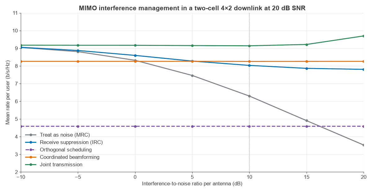
| Technique | INR 0 dB | INR 10 dB | INR 20 dB | Backhaul and CSI needs |
|---|---|---|---|---|
| Treat as noise | 8.32 | 6.30 | 3.53 | None |
| Receive suppression (IRC) | 8.59 | 8.03 | 7.81 | Interference covariance at the user |
| Orthogonal scheduling | 4.59 | 4.59 | 4.59 | Timing coordination |
| Coordinated beamforming | 8.26 | 8.26 | 8.26 | Cross-cell CSI |
| Joint transmission | 9.17 | 9.14 | 9.69 | Cross-cell CSI, shared data, phase coherence |
Rates are in b/s/Hz per user. Each row shows a different engineering trade:
- Treating interference as noise loses 58% between 0 and 20 dB INR.
- IRC is the cheapest large gain. A 2-antenna receiver can null one interferer and keep 7.81 b/s/Hz, and it needs nothing from the network.
- Coordinated beamforming costs 0.33 b/s/Hz against IRC at 0 dB and gains 0.45 b/s/Hz at 20 dB. It is independent of INR when CSI is perfect, and the crossing is near 5 dB.
- Orthogonal scheduling is safe and poor here, since half the time is a heavy price when antennas can do the same job. It is more attractive with few antennas or when channel knowledge is unavailable.
- Joint transmission turns interference into signal and rises slightly with INR, at the highest implementation cost.
A common pattern follows: use receive suppression everywhere, add transmit coordination where interference is strong and CSI is available, and reserve joint processing for clusters with fast, phase-coherent backhaul.
Effect of CSI error on interference management
Coordinated schemes depend on knowing a channel that belongs to someone else’s link. Repeating the coordinated beamforming case with error added to the cross-channel estimate at a normalised mean square error (NMSE) gives:
| CSI NMSE | Rate, INR 10 dB | Rate, INR 20 dB |
|---|---|---|
| Perfect | 8.26 | 8.26 |
| −20 dB | 8.13 | 7.68 |
| −10 dB | 7.68 | 7.12 |
Residual interference scales with INR multiplied by NMSE, so a strong interferer needs better CSI for the same result. At 20 dB INR, even −20 dB NMSE puts coordinated beamforming at 7.68 b/s/Hz, just below receive-only IRC at 7.81 b/s/Hz, and at that point the coordination has gained nothing. These figures keep the MMSE receiver in place, so the user’s antennas partly protect the link against those errors. Combining transmit and receive techniques is more tolerant of error than relying on either alone.
Interference management in practical systems
Cellular standards contain most of these ideas in constrained form. Static and soft frequency reuse, power control and almost-blank subframes are time and frequency coordination. Coordinated multipoint groups coordinated scheduling, coordinated beamforming and joint transmission under one framework. Advanced user receivers perform interference rejection, and network-assisted variants share interferer parameters so that a receiver can do better than suppression alone.
Massive MIMO shifts the balance. With many more antennas than users, fast fading between terminals averages out and uncorrelated interference falls with antenna count, leaving pilot contamination as the main residual. Pilot reuse planning then becomes an interference problem in its own right.
Wi-Fi MU-MIMO and uplink OFDMA follow the same logic with shorter coordination loops, while mmWave systems rely on narrow beams to provide much of the spatial isolation directly, as mmWave radio architectures describes.
Choosing an interference management approach
| Situation | First choice | Why |
|---|---|---|
| Interference well below signal | Treat as noise with link adaptation | Gains do not justify overhead |
| One or two dominant interferers, spare receive antennas | IRC or MMSE receiver | No network cost |
| Strong interference, fresh CSI, more transmit antennas than users | Coordinated beamforming | Keeps full-time use of the band |
| Dense cluster, fibre backhaul | Joint transmission | Turns interference into signal |
| Interferer far stronger than signal | Decode and subtract | See interference cancellation |
| No CSI, few antennas | Orthogonal resources | Simple and predictable |
Frequently asked questions
What is interference management in MIMO?
It is the set of receiver, transmitter and network techniques that control unwanted signals in a multi-antenna system. They include treating interference as noise, spatial suppression, cancellation, nulling, scheduling, interference alignment and joint transmission. The goal is the best use of spatial dimensions across a network, not simply the removal of all interference.
Is it better to suppress interference at the transmitter or the receiver?
Receiver suppression needs no network coordination and works against any spatially distinct interferer, so it comes first. Transmit nulling protects users that cannot suppress for themselves and saves their receive dimensions, but it needs CSI for the victim’s channel. Systems commonly use both.
What is interference alignment?
It is a transmit precoding method that packs interference at each receiver into a reduced subspace, leaving the rest free for wanted signals. With K users and N antennas per node, it gives a theoretical KN/2 degrees of freedom at high SNR. Its CSI demands limit practical use.
How many interferers can a MIMO receiver reject?
An N-antenna receiver can fully null up to N − 1 spatially independent streams, while receiving one stream of its own. In practice, depth is limited by estimation errors and by correlation between the interferer and wanted signal directions.
Related topics
The techniques on this page connect to beamforming, MIMO precoding and MIMO detection algorithms. See MIMO capacity for the rate limits they work toward and MIMO, beamforming and phased-array architectures for the hardware. Noise as the reference level for all of this is covered under RF noise, and the wider topic map is at RF design.