


Massive MIMO spectral efficiency is the data rate a large antenna array delivers per hertz of bandwidth, summed over all the users it serves at once. With 64 antennas serving 8 users at 0 dB SNR, zero forcing gives about 37 b/s/Hz, where a single-antenna link gives 1 b/s/Hz. The gain comes from sending many streams in the same bandwidth, and pilot overhead and pilot contamination set the limit.
This page calculates that number and shows what recent advances in massive MIMO systems are trying to improve. The general theory of multiple antennas is on the MIMO and multiple antenna systems page, and MIMO capacity covers the point-to-point limit. The transceiver hardware is in MIMO, Beamforming and Phased-Array Architectures.
What makes a massive MIMO system different
A massive MIMO base station has many more antennas than the users it serves in one time-frequency slot. M is the antenna count and K the number of users, and an M/K of about 3 to 10 is often quoted as a rule of thumb, not a hard limit. Commercial sub-6 GHz radios with 32 or 64 transmit and receive chains are typical. Each user usually has one to four antennas.
Two effects follow from M being large. Channels to different users become nearly orthogonal, so simple linear processing separates them. The channel also hardens: the beamforming gain varies far less from one fading block to the next, so the rate stays close to its average and the scheduler does not have to chase fades.
How massive MIMO spectral efficiency is calculated
Time and frequency divide into coherence blocks of τc symbols over which the channel is roughly constant. In TDD, K orthogonal pilots take τp = K of those symbols, and the rest carry data. Assuming independent Rayleigh fading, equal path loss, SNR ρ per user and MMSE channel estimation, the estimate holds a fraction of the channel power:
γ = τpρ / (1 + τpρ)
Standard uplink rate expressions for maximum ratio (MR) and zero forcing (ZF) combining then give the SINR per user:
SINRMR = Mργ / (1 + Kρ)
SINRZF = (M – K)ργ / (1 + Kρ(1 – γ))
The sum spectral efficiency applies the pilot overhead to all K users:
SE = K (1 – τp/τc) log2(1 + SINR)
These forms ignore neighbouring cells. MR treats the other users as noise, which is why its denominator grows with Kρ. ZF removes them, apart from the part it cannot see, which is the estimation error (1 – γ).
Worked example: 64 antennas and 8 users
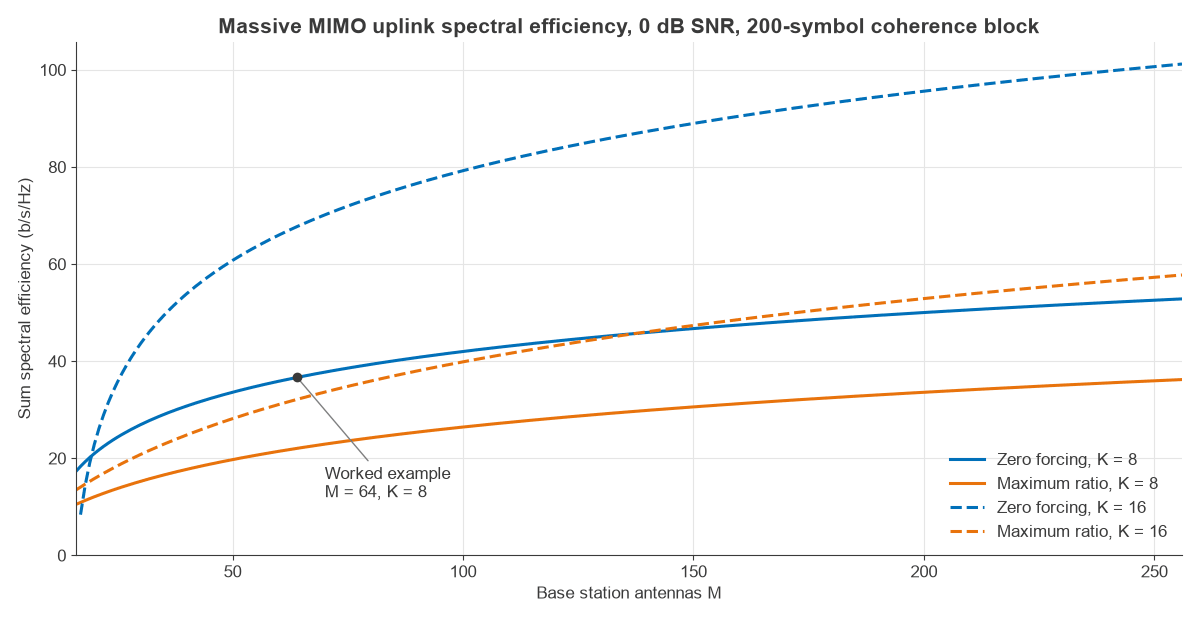
Take M = 64, K = 8, ρ = 0 dB (a linear value of 1) and τc = 200 symbols. The eight-symbol pilot gives γ = 8/9 = 0.889, and the overhead factor is 1 – 8/200 = 0.96.
- MR: SINR = 64 × 0.889 / 9 = 6.32, or 8.0 dB. Each user gets 0.96 log2(7.32) = 2.76 b/s/Hz, so the sum is 22.1 b/s/Hz.
- ZF: SINR = 56 × 0.889 / (1 + 8 × 0.111) = 26.4, or 14.2 dB. Each user gets 4.58 b/s/Hz, so the sum is 36.7 b/s/Hz.
A Monte Carlo simulation of the same link returned 8.0 dB and 14.2 dB, agreeing with both formulas. In 100 MHz of bandwidth, 36.7 b/s/Hz is about 3.7 Gb/s. A single-antenna link at the same 0 dB SNR gives log2(2) = 1 b/s/Hz, or 100 Mb/s.
| Antennas M | Users K | MR sum (b/s/Hz) | ZF sum (b/s/Hz) | ZF SINR (dB) |
|---|---|---|---|---|
| 64 | 8 | 22.1 | 36.7 | 14.2 |
| 64 | 16 | 32.1 | 67.7 | 13.7 |
| 128 | 16 | 44.4 | 85.2 | 17.3 |
Spectral efficiency grows mainly with K, because each added user is a new stream. Going from 8 to 16 users at M = 64 nearly doubles the ZF sum, while extra antennas only raise the SINR of existing streams, which adds logarithmically.
Pilot overhead and the best number of users
Serving more users cannot go on forever, because each user needs a pilot symbol taken from data. With τp = K, the overhead term (1 – K/τc) falls as the stream count rises. Optimising K for this model gives 42 users at M = 64 (118 b/s/Hz), 75 users at M = 128 (224 b/s/Hz) and 93 users at M = 256 (316 b/s/Hz).
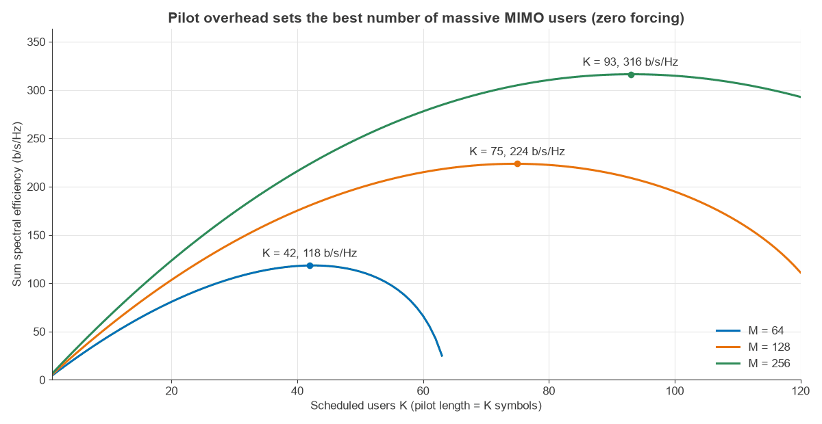
These optima are ceilings from an idealised model. Real channels are spatially correlated, users cluster, and few cells have 42 users ready to transmit in the same slot. Fast movers shorten τc, which pulls the optimum down.
Pilot contamination: the limit antennas cannot remove
Orthogonal pilots cannot stretch across a whole network, so cells reuse them. When a neighbouring user sends the same pilot, the base station’s channel estimate mixes the two users, and its beam points partly at the neighbour. Adding antennas sharpens that wrong beam as well as the right one, so this interference grows with M at the same rate as the signal.
For MR with neighbour-cell relative path gains αi, the SINR tends to a limit as M grows:
SINRlimit = 1 / Σαi2
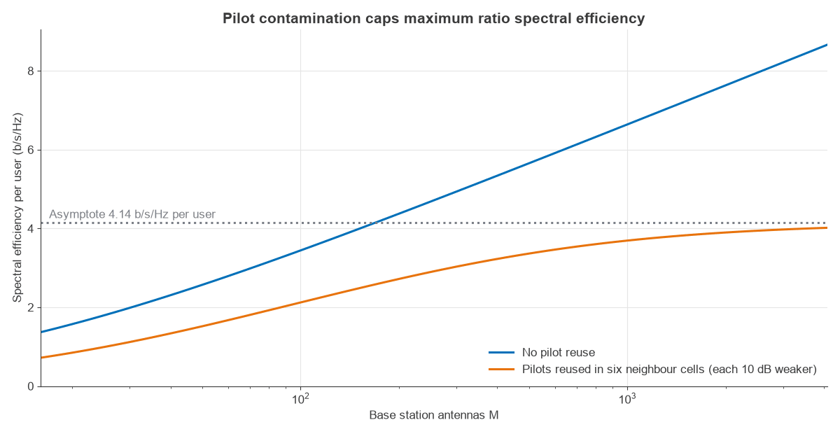
Take six neighbours, each 10 dB weaker in power (α = 0.1). The sum is 6 × 0.01 = 0.06, the limit is 16.7 (12.2 dB), and spectral efficiency per user cannot pass log2(17.7) = 4.14 b/s/Hz however many antennas are added.
| M | No pilot reuse (b/s/Hz) | Pilots reused (b/s/Hz) |
|---|---|---|
| 64 | 2.87 | 1.73 |
| 256 | 4.72 | 2.91 |
| 1024 | 6.67 | 3.70 |
The reused-pilot column also counts data interference from the same six cells, which the no-reuse column leaves out, so at small M part of the gap comes from that interference and not from contamination. The asymptote is a result for MR under this simple statistical model. Later work showed that multi-cell MMSE processing, combined with spatial correlation, can avoid a hard ceiling, which is one reason the topic stays active.
Advancements in massive MIMO systems
Most recent progress in massive MIMO spectral efficiency targets one of the terms in the equations above.
- Better processing. Regularised ZF and MMSE combining suppress interference more evenly than plain ZF, particularly when M/K is small. MIMO detection algorithms covers the receivers, and MIMO precoding the downlink equivalents.
- Smarter pilots. Pilot reuse factors above one, power control and pilot assignment based on user location all reduce Σαi2.
- FDD operation. TDD reciprocity avoids most feedback. FDD needs downlink pilots and reports, so codebooks and deep learning CSI feedback aim to cut that cost.
- Hybrid arrays at mmWave. With hundreds of elements, a full digital chain per element costs too much power, so several elements share one chain. mmWave radio architectures sets out the trade.
- Cell-free massive MIMO. Many distributed access points jointly serve users, which evens out rates across the coverage area at the cost of fronthaul and synchronisation.
- Lower-resolution converters. Using fewer ADC bits per chain saves power. The quantisation noise is partly uncorrelated across antennas, so the array averages some of it out.
The chain count that raises spectral efficiency also multiplies DC power, calibration effort and digital interface data rate. The hardware has to be judged alongside the b/s/Hz figure, which is why many deployments stop at 32 or 64 chains.
Frequently asked questions
What is the spectral efficiency of massive MIMO?
It depends on M, K, SNR and the coherence block. An idealised 64-antenna array with 8 users at 0 dB SNR gives about 22 b/s/Hz with MR and 37 b/s/Hz with ZF. Field results are lower, because neighbouring cells, correlation and traffic all reduce the number of useful streams.
Why does massive MIMO increase spectral efficiency?
It sends several streams in the same time and frequency, and the large array separates them spatially. Sum rate grows almost linearly with the number of streams, but only logarithmically with SINR.
How many antennas does a massive MIMO system have?
There is no strict boundary. Sub-6 GHz base stations typically use 32 or 64 digital chains with more radiating elements behind them, and mmWave panels hold hundreds of elements but few digital chains. What matters is that M is several times larger than K.
Does pilot contamination still limit massive MIMO?
It remains a practical limit for simple processing, as the 4.14 b/s/Hz example shows. Better pilot assignment and multi-cell processing reduce it. How far depends on how correlated the channels are and how much coordination the network can afford.
Related topics
Massive MIMO builds on spatial multiplexing and beamforming, and its accuracy rests on channel state information. To see what imperfect estimates cost, read channel estimation errors and their impact on system performance. Choosing which users share a slot is covered in user scheduling in MIMO systems.