

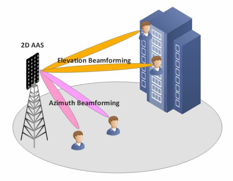
Beamforming techniques in cellular systems fall into two families: codebook methods, where the phone reports which pre-agreed beam suits it best, and reciprocity methods, where the base station measures the uplink and reuses that channel for the downlink. LTE and 5G NR use both, and 5G adds beam sweeping so that a mmWave cell can be found at all. Testing them means measuring the radiated beam over the air, because a modern array has no connector to probe.
The physics of the array is on the beamforming page, and the beginner route is MIMO beamforming basics. This page covers how a cellular network applies beamforming, what it costs in air-interface resources, and how the result is measured.
Why beamforming matters in cellular systems
A base station serves users whose positions it does not control, at the same time and on the same frequency as neighbouring cells. Beamforming helps in three ways. It raises SNR for users at the cell edge, cuts the interference spilled into other cells, and allows several users to share a slot (MU-MIMO). At mmWave it is mandatory, because a single element cannot close the link at useful range. The numbers behind those benefits are in the benefits of beamforming.
Types of beamforming techniques
The array can be built in three ways, and the network can choose its weights in several ways. These are separate choices.
| Technique | How weights are chosen | Typical use |
|---|---|---|
| Analog beamforming | One phase-shifted beam per chain, chosen from a set | mmWave user equipment and small panels |
| Digital beamforming | A complex weight per chain and per subcarrier | Sub-6 GHz 32T and 64T radios |
| Hybrid beamforming | Analog beams with digital weights across chains | mmWave base stations |
| Codebook-based | User reports a precoder index | FDD, and many TDD links |
| Reciprocity-based | Base station measures uplink sounding | TDD massive MIMO |
| Grid of beams | Fixed beams; user reports the best one | Control channels and mobile users |
The hardware trade between the first three is covered in MIMO, Beamforming and Phased-Array Architectures, and the weight calculations in MIMO precoding.
Beamforming techniques in LTE and 5G NR
Beamforming in LTE
LTE introduced user-specific beamforming through its transmission modes. Broadly, mode 7 carries one layer on a user-specific reference signal, mode 8 carries two, and mode 9 extends this to up to eight layers. Because the demodulation reference signal is precoded along with the data, the phone sees one combined channel and does not need to know the weights. That lets the base station use any precoder it likes, which is what makes reciprocity beamforming possible in TD-LTE.
Downlink beamforming in 5G NR
NR builds beams into its procedures from the start. Three signals do most of the work.
- SSB (synchronisation signal block). The cell’s initial beacon, sent as a sweep of wide beams.
- CSI-RS. Narrower reference signals that the phone measures to report the best beam, the rank and a precoder from a codebook. NR Type I codebooks are coarse and cheap, while Type II reports more detail for MU-MIMO at a higher feedback cost.
- SRS (sounding reference signal). Sent by the phone on the uplink. In TDD, the base station turns it directly into downlink weights.
Beam management then runs as three loops: a wide sweep to find a coarse direction, narrower base station beams to refine it, and refinement of the phone’s own beam. Channel state information describes how these estimates are formed and how fast they age.
Worked example: an SSB beam sweep
Take an 8-column array with half-wavelength spacing, covering a ±60 degree sector. The 3 dB beamwidth at broadside is about 0.886 × 2/N radians:
HPBW = 0.886 × 2/8 = 0.2215 rad, or 12.7 degrees
Beams widen when steered off boresight, but their width stays constant in sin(θ), so the beams are spaced uniformly in that variable. The sector spans sin(60°) – sin(-60°) = 1.732, and 1.732/0.2215 = 7.8, so 8 beams cover it. They point at ±6.4, ±19.4, ±33.6 and ±50.8 degrees, which fits the limit of about 8 SSB beams usually quoted for mid-band NR. Typical limits are about 4 at low frequency and 64 at mmWave.
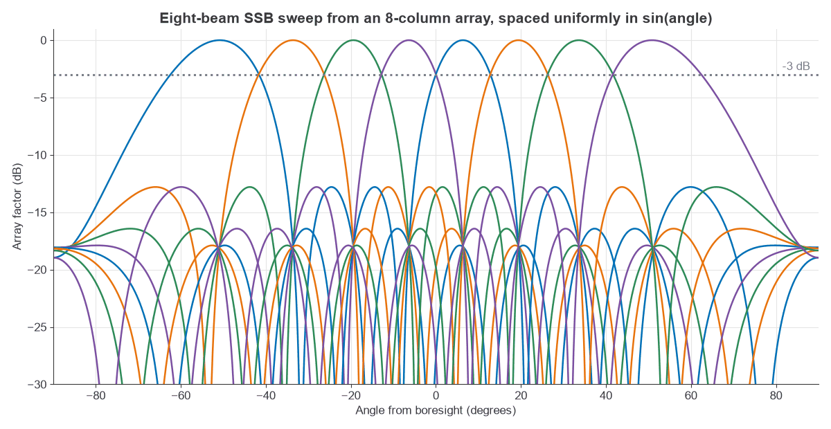
Now the cost. Each SSB takes 4 OFDM symbols and 240 subcarriers. With 30 kHz subcarrier spacing, the default 20 ms period holds 40 slots of 14 symbols, which is 560 symbols.
- Time used: 8 × 4 = 32 symbols of 560, or 5.7% of symbols.
- Resource elements used in a 100 MHz carrier (273 resource blocks, 3,276 subcarriers): 32 × 240 / (560 × 3,276) = 0.42%.
- Sweep duration on air: 32 × 35.7 µs = 1.14 ms.
- Search time: a phone trying 4 of its own beams, one per burst, covers all 8 × 4 = 32 pairs in 4 × 20 = 80 ms.
The overhead is small at this size, and it scales with the beam count. A 64-beam mmWave sweep costs eight times the symbols, though mmWave numerology shortens each one. The 80 ms search shows why a narrow-beam phone needs help during fast handover, and why the period and beam count are tuned for each deployment.
Reciprocity or feedback?
In TDD the uplink and downlink share a frequency, so the air channel is the same in both directions. The base station can derive weights from SRS and avoid feedback, which suits large arrays because the cost does not grow with M. It needs calibration of transmit and receive chains, because the RF paths are not reciprocal even when the air is. It also needs enough uplink power: a cell-edge phone may not deliver a clean SRS, and then the network can fall back on codebook reports.
In FDD the two directions use different frequencies, so the fading differs. The phone must measure and report, and the cost grows with the antenna count. See deep learning CSI feedback for how that report can be compressed.
Beamforming test and antenna measurement
A beamforming test confirms that a device forms the intended beam, points it in the right direction and keeps sidelobes down. Integrated arrays have no RF connector at each element, so nearly all of this is over-the-air (OTA) measurement. The main quantities are:
- EIRP, the radiated power in the beam direction, and its scan loss across angles.
- EIS, the receive sensitivity expressed as power at the array.
- Beam pointing error, the angle between the intended and measured peak.
- Sidelobe level and null depth, which show how good the calibration is.
- EVM over the air, measured in the beam. See measuring radio performance.
A useful check is the array’s EIRP budget. A 256-element array with 10 dBm per element and 5 dBi elements has:
EIRP = 10 + 10 log10(256) + 10 log10(256) + 5 = 63.2 dBm
The element count appears twice: once for total power and once for array gain. If the measured value is 3 dB low, some elements may be off or the phases may be wrong. Pattern shape helps tell these apart.
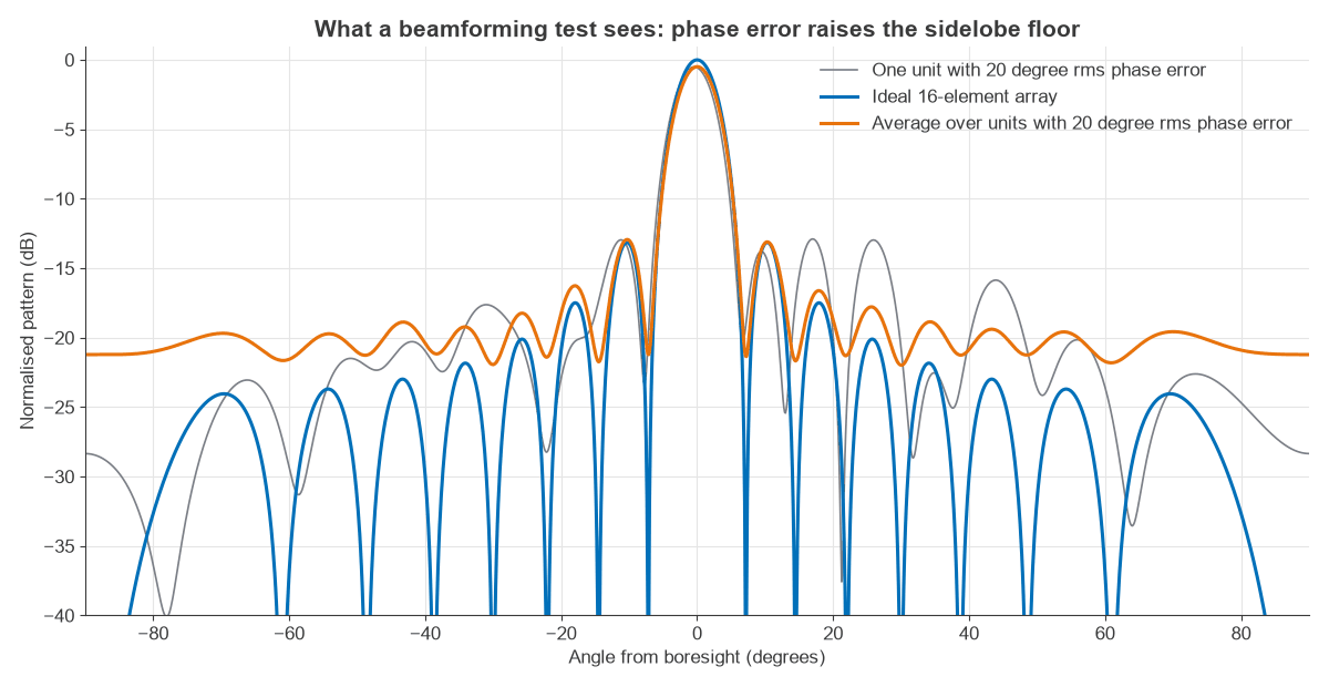
Peak gain hides phase errors well. The average loss is exp(-σ2) with σ in radians, which gives 0.03 dB at 5 degrees rms, 0.13 dB at 10 degrees, 0.53 dB at 20 degrees and 1.19 dB at 30 degrees. The energy lost from the peak goes into a raised sidelobe floor, which damages interference nulling far more than a half-decibel link loss suggests. A beamforming antenna measurement should therefore capture the whole pattern, not only the peak.
Choosing a test method
The far-field distance sets the method:
R = 2D2/λ
For a 16 × 16 array at 28 GHz, the side is D = 8λ = 85.7 mm, so R = 1.37 m, which fits a compact chamber. Taking D as the aperture diagonal, 121 mm, doubles that to 2.7 m. Free-space path loss over that distance is 64.1 dB, leaving about -1 dBm at a 0 dBi probe from the 63.2 dBm array above. A 0.6 m sub-6 GHz panel at 3.5 GHz needs 8.4 m, which means a much larger chamber.
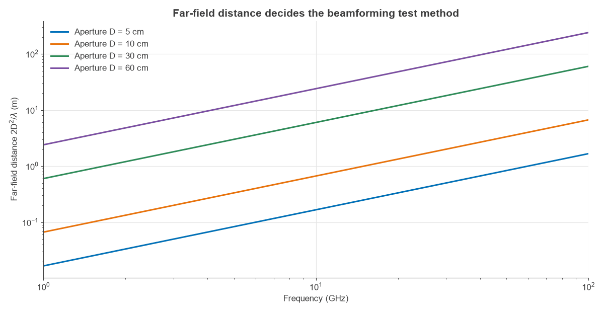
Direct far-field chambers suit small apertures. A compact antenna test range (CATR) uses a reflector to create a plane wave in a short distance. Near-field scanning samples close to the array and transforms the data to the far field, which handles big arrays at the cost of scan time.
Frequently asked questions
What are the main types of beamforming?
By hardware, they are analog, digital and hybrid. By how weights are chosen, they are codebook, reciprocity and grid of beams. Cellular networks mix them: 5G usually sends SSB on a grid of beams and data on narrower reciprocity or codebook beams.
Is beamforming used in LTE?
Yes. LTE supports user-specific beamforming through transmission modes such as 7, 8 and 9, and codebook precoding in other modes. It works with few antennas compared with 5G NR, so the gain is more modest.
How do you test beamforming?
Point the device’s beam at a measurement probe in an anechoic chamber or CATR, then scan angles and record EIRP, pattern and EVM. Repeat across beams and frequency. A conducted test is only possible where the design exposes RF ports.
What is the difference between beamforming and MIMO?
Beamforming focuses one stream using many antennas. MIMO is the wider idea of using many antennas at both ends, and it may also send several streams. A cellular link often does both at once. The MIMO beamforming basics page explains the difference with a small example.
Related topics
For hardware, see phased array design and the 5G RF front end. Massive MIMO spectral efficiency shows what these techniques achieve at scale, and antenna parameters defines the gain and beamwidth terms used here.