

Beamforming combines the signals of an antenna array with chosen phase and amplitude weights, so that they add constructively in one direction and cancel in others. On transmit this concentrates radiated power toward the receiver, and on receive it raises SNR and suppresses interference. An array of N elements gives up to 10 log10(N) dB of array gain, plus the ability to steer electronically with no moving parts.
This article works through the array factor, beam steering and its limits in RF hardware. It is part of the MIMO group: MIMO and multiple antenna systems gives the overview, spatial multiplexing covers parallel streams, and MIMO, Beamforming and Phased-Array Architectures covers the transceiver architectures.
Array factor of a uniform linear array
Consider N identical elements in a line with spacing d. A plane wave arriving at angle θ from broadside reaches each successive element with an extra phase of (2πd/λ) sin θ. If element n is given a weight with phase -nβ, where β = (2πd/λ) sin θ0, the signals align exactly when θ = θ0. With equal amplitudes, the normalised array factor is:
|AF(θ)| = |sin(Nψ/2) / (N sin(ψ/2))|, where ψ = (2πd/λ)(sin θ – sin θ0)
The total pattern is the array factor multiplied by the element pattern. Three approximate results follow for half-wavelength spacing:
- Phase step: β = 180° x sin θ0. Steering to 15° needs 46.6° per element, 30° needs 90.0° and 45° needs 127.3°.
- Half-power beamwidth: approximately 0.886 λ/(Nd cos θ0) radians. The beam widens as it scans, because the projected aperture shrinks.
- First sidelobe: about -13 dB with uniform weights, whatever the array size.
Worked example: a 16-element array at 28 GHz
At 28 GHz, λ = 10.71 mm, so half-wavelength spacing is 5.35 mm. Assume 16 elements, each driven by a PA delivering 10 dBm into an antenna of 5 dBi peak gain. The element is assumed to have a cos θ power pattern.
| Quantity | Calculation | Result |
|---|---|---|
| Total conducted power | 10 dBm + 10 log10(16) | 22.04 dBm |
| Array gain | 10 log10(16) | 12.04 dB |
| EIRP at broadside | 10 dBm + 20 log10(16) + 5 dBi | 39.08 dBm |
| Element scan loss at 30° | 10 log10(cos 30°) | -0.62 dB |
| EIRP at 30° | 39.08 dBm – 0.62 dB | 38.46 dBm |
| Beamwidth at broadside | Numerical, formula gives 6.35° | 6.36° |
| Beamwidth at 30° | Numerical, formula gives 7.33° | 7.35° |
| Receive SNR gain | Independent noise per chain | 12.04 dB |
Note the 20 log10(N) term. EIRP gains twice when each element has its own PA: once from N times the conducted power, and once from N times the array gain. A receive array gets the 10 log10(N) term only. These figures feed directly into a link budget, and antenna parameters covers the distinction between directivity and gain.
Amplitude tapering and sidelobes
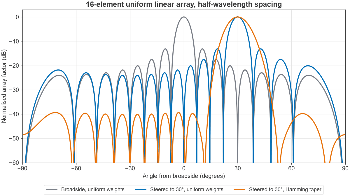
A -13 dB sidelobe is often too high, since it can leak energy toward other users or admit interference. Tapering the amplitude toward the edges of the array lowers sidelobes, at the cost of a wider main beam and some lost gain. For the 16-element array, a Hamming taper produces these results, also plotted in Figure 1:
| Weighting | Peak sidelobe | Beamwidth (broadside) | Taper loss |
|---|---|---|---|
| Uniform | -13.1 dB | 6.36° | 0 dB |
| Hamming | -39.4 dB | 9.74° | 1.54 dB |
On transmit, tapering has a further cost. Backing off the outer PAs means they are used below their rated output, so EIRP and efficiency both fall. On receive, tapering is cheap because it can be applied digitally or in a gain stage after the LNA.
Grating lobes and element spacing
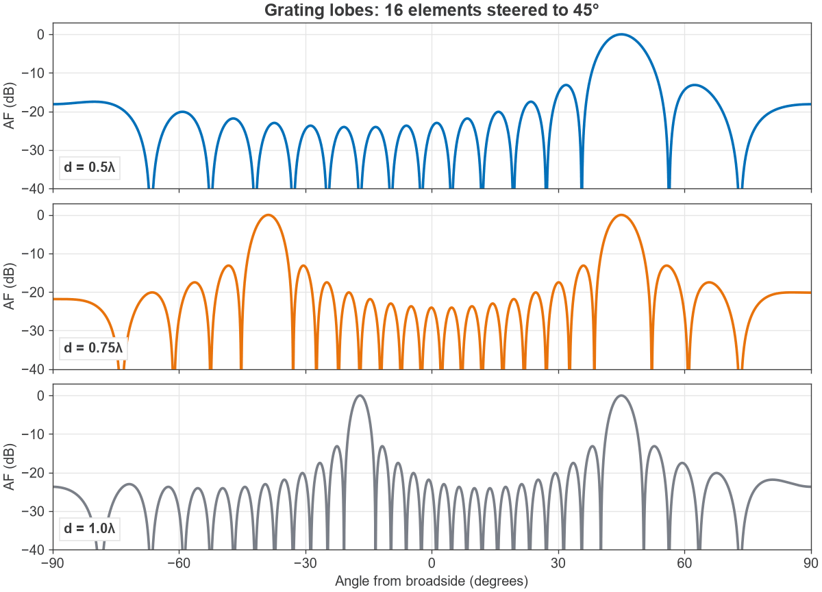
Spacing beyond a certain limit produces additional full-size beams, called grating lobes, because the phase across the aperture becomes ambiguous. They appear where sin θg = sin θ0 – mλ/d for integer m. To keep them out of visible space:
d/λ < 1 / (1 + |sin θmax|)
| Maximum scan angle | Maximum spacing |
|---|---|
| 30° | 0.667λ |
| 45° | 0.586λ |
| 60° | 0.536λ |
Figure 2 shows the effect at 45° scan. At 0.5λ there is one beam. At 0.75λ a second full beam appears at -38.8°, and at 1.0λ it moves in to -17.0°. Half-wavelength spacing avoids the problem entirely, which is why it is the common default. At wider spacing, a directive element pattern helps to suppress grating lobes, though it also limits scan range.
Analog, digital and hybrid beamforming
The architectures differ in where the weights are applied. This choice sets cost, power and flexibility.
| Architecture | Where weights apply | Simultaneous beams | Main cost |
|---|---|---|---|
| Analog | RF or LO phase shifters | One per RF chain | Phase-shifter loss, limited agility |
| Digital | Baseband, per element | Many | One converter pair and chain per element |
| Hybrid | Both, in sub-arrays | A few, one per digital chain | Calibration and design complexity |
Analog beamforming applies one weight across the whole band, which limits it to one beam per chain. Digital beamforming gives per-subcarrier weights and any number of beams, but the data rate and converter power scale with element count. Hybrid designs are common at millimetre-wave frequencies, where the arrays are large. See mmWave radio architectures for those designs.
Interference nulling
Beamforming can also steer nulls. To protect a user at direction ai while serving direction ad, project the desired steering vector onto the space orthogonal to the interferer:
w = ad – ai (aiH ad) / N
The main-beam loss from this operation is 10 log10(1 – c2), where c is the conventional array response in the interferer’s direction. For the 16-element array serving broadside:
| Interferer angle | Conventional rejection | Main-beam loss with null |
|---|---|---|
| 4° (inside main beam) | -5.0 dB | 1.65 dB |
| 8° (just past the first null) | -20.0 dB | 0.04 dB |
The null is exact in these calculations. In hardware, its depth is limited by calibration, phase-shifter resolution and channel knowledge. An interferer inside the main beam can be nulled, but only by paying noticeable gain.
Hardware limits on beamforming
Phase-shifter resolution
A b-bit phase shifter leaves an error of up to half a step. Treating this error as uniformly distributed, the mean gain loss is 20 log10(sinc(1/2b)), where sinc(x) = sin(πx)/(πx). The table gives both this result and a Monte Carlo check.
| Bits | Step | Mean gain loss (formula) | Monte Carlo |
|---|---|---|---|
| 2 | 90° | 0.91 dB | 0.91 dB |
| 3 | 45° | 0.22 dB | 0.22 dB |
| 4 | 22.5° | 0.06 dB | 0.06 dB |
| 6 | 5.625° | 0.003 dB | 0.003 dB |
Gain loss is rarely the deciding factor. Coarse phase resolution matters more for sidelobes and null depth, and the periodic error from quantisation can form distinct lobes.
Calibration and phase error
Random phase errors of RMS σ radians reduce gain by about e-σ². That is 0.03 dB at 5° RMS, 0.13 dB at 10° and 0.53 dB at 20°. Gain is forgiving, but nulls and low sidelobes are not. Practical arrays need calibration across frequency, temperature and gain state.
Phase noise and noise figure
The array SNR gain assumes uncorrelated noise. LNA noise satisfies this, since each element has its own device, so the first stage sets the system noise temperature. Phase noise from a shared LO is common to every element, so it is not averaged down by combining. It sits on the combined signal just as it would on one element.
Beam squint and true time delay
A phase shifter gives a fixed phase, whereas an arriving wavefront needs a fixed delay. Away from the design frequency f0, the beam moves to:
sin θ = (f0/f) sin θ0
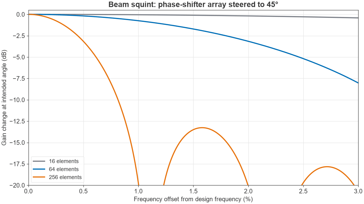
Steering to 45° at 28 GHz and operating at 28.4 GHz (a 1.43% offset) moves the beam to 44.20°, a shift of 0.80°. The effect depends on beamwidth, so it depends on array size:
| Elements | Beamwidth at 45° | Gain change at 28.4 GHz |
|---|---|---|
| 16 | 9.03° | -0.09 dB |
| 64 | 2.24° | -1.55 dB |
| 256 | Narrower than the shift | -14.2 dB |
The cure for large wideband arrays is true time delay. Each element is delayed by nd sin θ0/c. For the 28 GHz array steering to 30°, that step is 8.93 ps per element, or 133.9 ps across the 16-element aperture. Digital arrays can apply this per subcarrier.
Beamforming in multipath channels
The array factor describes a beam aimed at one direction, which suits line-of-sight links. In multipath the best weights do not form a clean beam: maximum ratio transmission uses the conjugate of the measured channel at each element, so several reflected paths add in phase at the receiver. The two views agree in line of sight. Analog systems usually find a beam by training through a codebook of about N beams to cover a sector, while digital systems can estimate the channel directly. Wider use of the channel is described under spatial multiplexing.
Frequently asked questions
What is the difference between beamforming and a phased array?
A phased array is hardware: a set of antenna elements with controllable phases. Beamforming is the process of choosing the weights. A phased array usually beamforms by phase alone, whereas digital beamforming can set the amplitude and phase of each element for each frequency.
How much gain does beamforming add?
Ideally 10 log10(N) dB of array gain, so 12 dB for 16 elements. EIRP grows as 20 log10(N) dB when each element has its own PA. Scan loss, taper loss and phase errors reduce both. The examples on this page (30° scan, Hamming taper, 3-bit phase shifters) add up to about 2.4 dB.
Why is half-wavelength spacing used?
It keeps grating lobes out of visible space at every scan angle, while packing as many elements as possible into an aperture. Wider spacing gives a narrower beam for the same element count, but only by limiting scan range. Narrower spacing increases mutual coupling.
Does beamforming work with only two antennas?
Yes. Two elements give 3 dB of array gain and can place one null. The beam is broad, so the benefit is mostly in SNR and not in spatial selectivity. Each added element gives one more degree of freedom.
Related topics
MIMO and multiple antenna systems places beamforming among diversity and multiplexing, and spatial multiplexing extends it to several streams. MIMO, Beamforming and Phased-Array Architectures covers transceiver design, with a separate 64-element example. The antennas hub collects element design and propagation.